17
$\begingroup$

I have this algorithm which I encountered:

(1) Generate $U_1$, $U_2$ independently from Uniform(0,1)

(2) Set $Y_1 = -\log{U_1}, Y_2 = -\log{U_2}$. If $Y_2 > \frac{(1-Y_1)^2}{2}$, accept $(Y_1, Y_2)$. Else reject and return to step 1.

(3) Generate $U_3$ from Uniform(0,1). If $U_3 < 0.5$, accept $X=Y_1$. Else, $X=-Y_1$


Why does X follow a standard normal distribution in the end? I know $Y_1$ and $Y_2$ here are exponential R.Vs. I probably need to understand how comparing $Y_2$ and $\frac{(1-Y_1)^2}{2}$ here does the trick and the third step is probably the result of a distribution formed after step 2 which is a folded standard normal distribution.

Edit: Source: Class Notes on Monte Carlo Methods

$\endgroup$
11
  • 2
    $\begingroup$ Step (2) draws a value of $Y_1$ conditional on $Y_2\gt(1-Y_1)^2/2.$ Find the chance that this value is less than or equal to $z$ by integrating the joint density. $\endgroup$
    – whuber
    Commented Sep 2, 2022 at 17:03
  • 3
    $\begingroup$ And the answer is columbia.edu/~ks20/4703-Sigman/4703-07-Notes-ARM.pdf (Note that this is not a great algorithm to generate Normals.) $\endgroup$
    – Xi'an
    Commented Sep 2, 2022 at 18:04
  • 3
    $\begingroup$ @Xi'an Right. Partially compensating for the need for almost 3 uniforms per variate is the relative simplicity of the calculations. But I understand now what you were referring to. What appeals to me about this approach is its potential to generate variates from analytically less-tractable distributions. $\endgroup$
    – whuber
    Commented Sep 2, 2022 at 18:28
  • 4
    $\begingroup$ Please edit your question to credit the original source of all material written by others (e.g., your screenshot): stats.stackexchange.com/help/referencing $\endgroup$
    – D.W.
    Commented Sep 3, 2022 at 19:18
  • 1
    $\begingroup$ Note that this doesn't really require 2.64 uniform samples - the last one only requires sampling one random bit, since you're only interested in the truth value of the expression (U3 < 0.5). Purely theoretically, you can take a single uniform sample X to generate U_1 = 2X (modulo 1) and U_3 = X, and you will have that the variables U_1 and (U_3 < 0.5) are independent. In practice, computationally speaking you are probably generating floating-point numbers in the range [0, 1) which involves generating 64 random bits and only using 53 of them, so the extra bit is free. $\endgroup$
    – kaya3
    Commented Sep 4, 2022 at 13:58

2 Answers 2

20
$\begingroup$

I was wondering how anyone would come up with this idea.

You observe, correctly, that the $Y_i$ have exponential distributions. They were easy to generate from a standard uniform number generator. The question could be put like this:

Find a simple way to exploit your ability to generate $(Y_1,Y_2)$ to draw values $Z$ following any continuous distribution with positive support.

Such a distribution is one with a density function proportional to $e^{g(z)}$ for a function $g$ defined on the positive numbers.

The key terms "simple" and "proportional to" suggest trying a rejection sampling method. That leads to the algorithm in the question in the following generalized form:

Generate $(Y_1,Y_2)$ and keep $Y_1$ provided $Y_2 \gt f(Y_1)$ for some function $f$ to be determined.

Although it might feel more natural to reject when $Y_2\le f(Y_1),$ as we will see this equivalent formulation leads to a simple calculation.

The result of this sampling procedure evidently produces values of $Y_1$ conditional on the event $Y_2 \gt f(Y_1).$ To find its distribution function, apply the (elementary) definition of conditional probability to the event $Y_1 \le z$ for an arbitrary positive number $z.$ It states

$$\Pr(Y_1\le z \mid Y_2 \gt f(Y_1)) \ \propto\ \Pr(Y_1\le z\text{ and }Y_2 \gt f(Y_1)).$$

We needn't be concerned about the constant of proportionality because we can work it out at the very end, knowing the result has to evaluate to $1$ as $z\to\infty$ (by the axiom of Total Probability).

Because $(Y_1,Y_2)$ is independent, their joint density is exponential. Thus, assuming $f(z) \ge 0$ for all $z\gt 0,$

$$\begin{aligned} \int_0^z e^{g(y_1)}\,\mathrm{d}y_1 &= \Pr(Y_1\le z\text{ and }Y_2 \gt f(Y_1)) \\ &\propto \int_0^z e^{-y_1}\int_{f(y_1)}^\infty e^{-y_2}\,\mathrm{d}y_2\mathrm{d}y_1\\ &= \int_0^z e^{-y_1 - f(y_1)}\,\mathrm{d}y_1. \end{aligned}$$

Equality will hold for all $z$ provided the two integrands are equal. Solving for $f$ gives

$$f(z) = -z - g(z) + C$$

where the number $C$ accounts for the neglected proportionality constant $e^C.$

Consider the Half Normal distribution where $g(z) = -z^2/2.$ We find

$$f(z) = -z + z^2/2 + C = (1 - z)^2/2 + C - 1/2.$$

We will need $C \ge 1/2$ to assure $f(z)$ is nonnegative. Larger values of $C$ work, too, but cause more rejections and are thereby less efficient.

Clearly, step (3) in the question converts any positive variable (like a Half Normal variable) into a variable symmetrically distributed around $0.$

Applications

For this method to succeed, we need $f$ to attain a minimum that is not too negative. This implies the target distribution must not be too heavy-tailed. One example is the generalized Gamma distribution with density proportional to $\exp(-z^3/3)$ on the positive numbers.

Here are histograms based on a million draws of $(Y_1,Y_2)$ for the Half Normal and Generalized Gamma problems. The red curves plot the target densities to demonstrate the correctness of this algorithm. The (empirical) acceptance rates show how efficient it is.
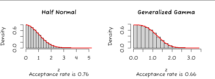
enter image description here

This R code produced these plots.

set.seed(17)
n <- 1e6
Y <- matrix(-log(runif(2*n)), ncol = 2) # Step (1): obtain iid exponential variates
#
# The function `f`.  The constant can be any non-negative value, with 0 being the
# most efficient.
#
Dists <- list(`Half Normal` =  function(z, C = 0) (1 - z)^2/2 + C,
              `Generalized Gamma` = function(z, C = 0) -z + z^3/3 + 2/3 + C)
pars <- par(mfrow = c(1, length(Dists)))
for(D in names(Dists)) {
  f <- Dists[[D]]
  z <- Y[Y[, 2] > f(Y[, 1]), 1]  # Step (2) of the rejection sampling
  rate <- length(z) / nrow(Y)

  hist(z, freq = FALSE, main = D, 
       sub = bquote(paste("Acceptance rate is ", .(signif(rate, 2)))))
  g <- function(x) exp(-x - f(x))

  A <- integrate(g, 0, Inf)$value # The constant of integration
  curve(g(x) / A, add = TRUE, col = "Red", lwd = 2)
}
par(pars)
$\endgroup$
4
  • 2
    $\begingroup$ (+1) Very nice reverse engineering. Historically von Neumann started by dominating the half-Normal density with a standard Exponential density and then achieved this condensed version. $\endgroup$
    – Xi'an
    Commented Sep 2, 2022 at 18:34
  • 2
    $\begingroup$ @Xi'an I have realized -- and checked in code -- that one can overcome the limitation on tail behavior by means of a suitable transformation such as a logarithm or root. For instance, to generate a Gamma$(a)$ variate use $f(z) = -(1+a)z + \exp(z) + C$ after finding $C$ through numerical optimization. For smallish $a$ the acceptance rate isn't bad; e.g. it's 66% for $a=0.3$ and 39% for $a=3.$ This makes the approach much more general than I had thought. $\endgroup$
    – whuber
    Commented Sep 2, 2022 at 18:47
  • $\begingroup$ @whuber Thank you! $\endgroup$
    – arcancor
    Commented Sep 3, 2022 at 6:54
  • 1
    $\begingroup$ A more natural way to come up with it: since going from Cartesian to polar gives$$\frac{1}{2\pi}e^{-(y_1^2+y_2^2)/2}dy_1dy_2=re^{-r^2/2}dr\frac{d\theta}{2\pi},$$it's now easy to get the desired IIDs viz. $u_1=e^{-y_1^2}$ (we can drop the $1-$ you'd get if you wanted an order-preserving transformation), $u_2=\theta/(2\pi)$. This speaks to a deeper truth: the only way for two Cartesian coordinates to be IIDs, with the polar coordinates also independent, is for the IIDs to be $N(0,\,\sigma^2)$. $\endgroup$
    – J.G.
    Commented Sep 4, 2022 at 20:44
6
$\begingroup$

To draw a comparison between this Normal generator (that I will consider as von Neumann's) and the Box-Müller polar generator,

#Box-Müller
bm=function(N){
  a=sqrt(-2*log(runif(N/2)))
  b=2*pi*runif(N/2)
  return(c(a*sin(b),a*cos(b)))
}

#vonNeumann
vn=function(N){
  u=-log(runif(2.64*N))
  v=-2*log(runif(2.64*N))>(u-1)^2
  w=(runif(2.64*N)<.5)-2
  return((w*u)[v])
}

here are the relative computing times

> system.time(bm(1e8))
utilisateur     système      écoulé 
     7.015       0.649       7.674 
> system.time(vn(1e8))
utilisateur     système      écoulé 
     42.483       5.713      48.222 
$\endgroup$
5
  • 1
    $\begingroup$ FWIW, vn does not return a Normal variate, nor does it return anywhere near N values. When it's fixed up, the relative timings are still about the same as you report. But when a better implementation of vn is used--you are welcome to borrow the one in my answer--the timing ratio is 3:1 (21:6.9). With a little optimization it drops to the expected 2.6:1, reflecting the RNG costs. vn <- function(N) { N <- ceiling(1.32 * N); y1 <- log(runif(N, 0, exp(1))); y2 <- -2 * log(runif(N)); y1 <- y1[y2 > y1^2]; sample(c(-1,1), length(y1), replace = TRUE) * (y1 - 1) } $\endgroup$
    – whuber
    Commented Sep 3, 2022 at 16:37
  • 1
    $\begingroup$ @whuber: thank you, issues fixed after a busy weekend... $\endgroup$
    – Xi'an
    Commented Sep 5, 2022 at 14:17
  • $\begingroup$ Why is this vn func only returning the left-hand half of a normal dist? While one could replace the output with K <- c(K,-K) , that gives an artificial perfect mirror, not what's desired. $\endgroup$ Commented Sep 15, 2022 at 11:51
  • $\begingroup$ Oh, -- you forgot the part " U3<0.5, accept X=Y1. Else, X=−Y1 " ... at least I think so. $\endgroup$ Commented Sep 15, 2022 at 12:16
  • $\begingroup$ @Xi'an then shouldn't it be w = ( (runif(2.64*N)<.5) -0.5) * 2 ? $\endgroup$ Commented Sep 15, 2022 at 18:02

Your Answer

By clicking “Post Your Answer”, you agree to our terms of service and acknowledge you have read our privacy policy.

Not the answer you're looking for? Browse other questions tagged or ask your own question.