Compute slopes for both levels of a factor

Question

Here is the linear mixed model that I am working with:

p3 <- lmer(respTime ~ proc*farFC+(1 | Subject), dtINT)

Proc refers to a factor with 2 levels (adjacent and overlay) farFC refers to a continous variable with 9 levels

The main output is below.

The slope of overlay is = 0.958.

When I change the reference level from adjacent to overlay, the slope of adjacent is -0.958.

Here is the code for how I am changing the reference level:

dtINT <- within(dtINT, proc <- relevel(proc, ref = 2)) 
#1 = ref level is overlay, 2 = ref level is adjacent

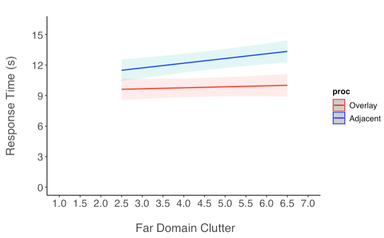
Why are the slopes the same but in opposite directions? Below is a graph, and we can see that the slopes are not the same (lines are not perfectly parallel).

How do I compute the slopes of each of these lines from the model? Said differently, how do I compute the slopes for each level of my IV? How do I tell if each of those slopes are significant?

Answer 1

You are mistaken about what your model parameters are. The fixed effects look like this: $$\beta_0 + \beta_11(\text{proc = Overlay}) + \beta_2\text{farFC} + \beta_31(\text{proc = overlay)}\cdot\text{farFC} $$

$1(x)$, being the indicator function. This means, that intecept = $\beta_0$ is the value at farF = 0 of the adjacent "group". procOverlay = $\beta_1$ marks the difference in intercept, which is why $\beta_1$ changes sign when you switch the reference level. The intercept will have also gone up by the same 0.958.

Now farFC = $\beta_2$ is your actual slope in the reference level and procOverlay:farFC = $\beta_3$ is the change in slope for the Overlay-"group".

Your regression lines are:

• Adjacent: $9.37 + 0.098\cdot x$, $x$ being the value of farFC, which starts at 2.5.
• Overlay: $9.37 + 0.958 + (0.098 + 0.365)\cdot x = 10.328 + 0.463\cdot x$

Now Adjacent is almost flat while Overlay is generally a bit higher and has a noticeable rise. This what you see in your plot except that your legend is the wrong way around. I'd assume, because you used the old model and the releveld data.

Now the difference between the two slopes is almost significant with the sign being identical, so the sum probably will be, but to check you can just fit releved data, where the new farFC will be 0.463. Keep in mind you are technically doing multiple comparisons.