Does this plot satisfy the linear regression model assumptions?

Question

Two assumptions of linear regression are:

1. Linearity: $E[Y_i|X_i] = \beta^{*t}X_i = E[\epsilon_i] = 0$

2. The variance is fixed and it isn't dependent on $i$. Or in other words, homoscedasticity.

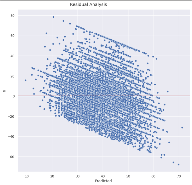
The simplest check is to plot the residuals ($e_i = Y_i - \hat{Y_i}$) as the Y-axis and the predicted values as the X-axis.

We expect:

1. From the linearity assumption: the residuals should be around the line e = 0.

2. From the constant variance assumption: similar spread of the residuals around the line = 0.

I've made such a plot. I found the predictions and the residuals with this code: (X are the predictive features and Y is the target feature).

predictions = X @ np.linalg.lstsq(X, Y, rcond=None)[0]
residuals = Y - predictions

And made the plot to check the two assumptions above, but I don't know how to interpret this plot. Does this mean that these two assumptions are reasonable? what can I infer about the spread of the residuals?

EDIT -

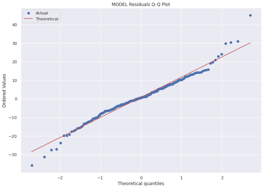
I've also made a Q-Q plot using the residuals in order to check the normality of the noise, using this code:

stats.probplot(residuals, dist="norm", plot= plt)
plt.title("MODEL Residuals Q-Q Plot")
plt.legend(['Actual','Theoretical']);

I got this:

I added this edit because I don't know if this has to do with the first plot. If it helps to interpret the first plot then here it is. Thanks!

Answer 1

Your plot shows that large predictions are on average too high (most residuals are negative) and small predictions are on average too small. So the assumption of linearity is proved false.

In such a case, to build a good quality model with a linear regression, you first need a non-linear transformation of the Y value. Is there any reason to expect that the underlying process is multiplicative rather than additive? If so, trying to predict $log(Y)$ is reasonable. More rarely, e.g. $\sqrt{Y}$ might be appropriate.