Null hypothesis significance testing, NHST, is expressing an observed effect in terms of a probabilistic comparison with the hypothesis of an absence of the effect. An observation is statistically significant if there is a clear distinction in the support of the data for absence versus presence of an effect.
An example of performing NHST with Bayesian techniques can be the following:
Imagine there is a lady that claims that she can taste whether the tea or the milk was first added to the cup. We would like to test that claim by having her perform a blind taste test.
We test the ability of the lady, by presenting her 100 cups of tea where she has to guess whether it was tea or milk first and we record the number of correct guesses. Let's for simplicity assume that the probability of a correct guess is symmetric (independent from whether the cup was tea first or milk first).
Say that based on prior information we know that there is a probability of 0.99 to have a person that can't taste anything (the null hypothesis), and a probability of 0.01 probability that a person can taste something and the ability of this person will follow a uniform distribution.
$$\begin{array}{RL}
H_0:&p=0.5\\
H_a:&p\sim U(0.5,1)
\end{array}$$
We have the following likelihoods as function of the number of heads:
$$\begin{array}{rcl}
\mathcal{L}(H_0,k) &=& {n \choose k} 0.5^n\\
\mathcal{L}(H_a,k) &=& \int_{0.5}^1 2 {n \choose k} p^{k}(1-p)^{n-k} dp
\end{array}$$
and a likelihood ratio (where we can compute the denominator with as the incomplete beta function)
$$
\Lambda = \frac{\mathcal{L}(H_0,k)}{
\mathcal{L}(H_a,k)} = \frac{1}{2^{n+1}\int_{0.5}^1 p^{k}(1-p)^{n-k} dp}$$
and posterior odds as function of $k$
$$
\frac{P(H_0;k)}{P(H_a;k)} = \frac{P(H_0)}{P(H_a)} \frac{\mathcal{L}(H_0,k)}{
\mathcal{L}(H_a,k)}
$$
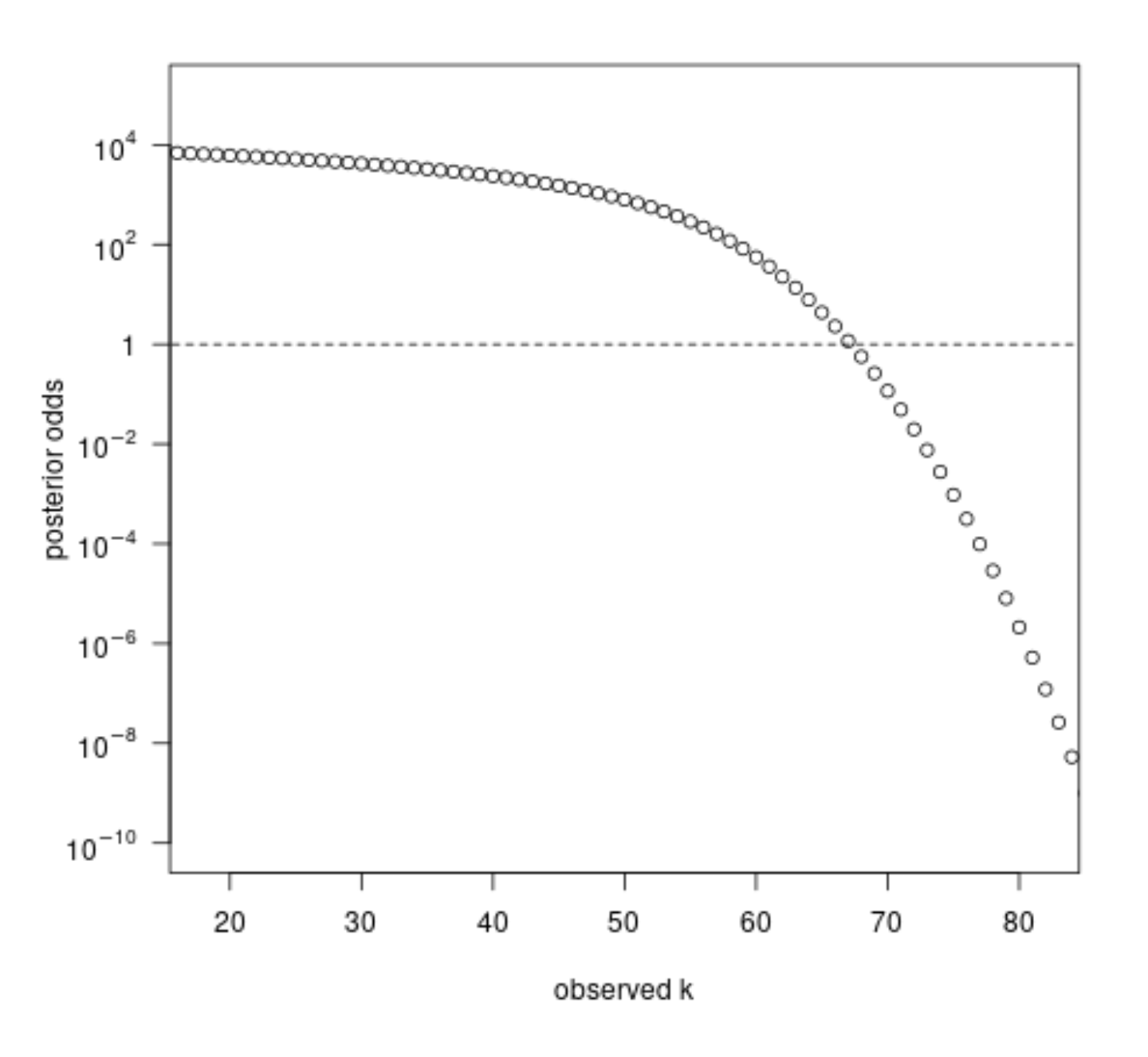
will look like

If for example the lady has two thirds (67) of the tea cups guessed correctly, then this indicates an effect that she can have more than half guessed correctly. But it is not significant. The null hypothesis is just as likely as the alternative hypothesis (odds ratio around one or even slightly above it).
The classical null hypothesis significance testing is not using these priors and are using instead probability statements based on a fiducial distribution or p-value.
Those statements are independent from a prior distribution (but not on prior information, e.g. assumptions about the model describing the likelihood function), and they only regard the likelihood of the null hypothesis and aim to make this a small value in order to declare a test statistically significant.
In a way the NHST has an implicit Bayesian reasoning and assumes that data that does not support the null hypothesis is supporting instead some alternative, but unknown, alternative hypothesis. Neyman and Pearson make this more explicit by defining the fiducial distribution or p-values (which can be computed in different ways) based on a specfic alternative hypothesis.
Possibly a more simple way to regard statistical significance, and how I interpret Fisher's approach to it, is that the fiducial distribution has a probability density concentrated in a small region (and in a Bayesian analysis one could use the posterior distribution in place of the fiducial distribution).
An effect is statistically significant if the highest density region (or some other region) of a certain large amount, say 95%, does not include the parameter value relating to a zero/null effect.
Expressions of statistical significance are useful when people make point estimates. A point estimate could for instance be the maximum of the posterior distribution. But such point estimate alone does not give an indication of the entire posterior and of the difference of the estimate with other hypotheses. If we give a point estimate along with a region, then we can have a better idea about the information that the data contains about a particular parameter/hypothesis.

