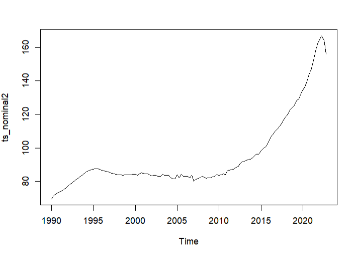
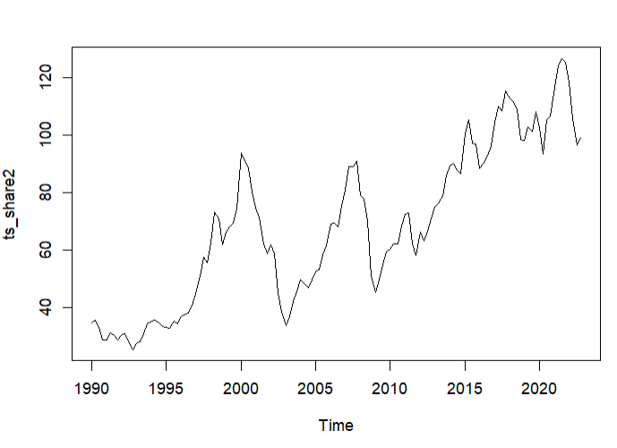
For my Master thesis I have to perform the DCC-GARCH model to examine the correlation between real estate house prices and the stock market. I tested the data for normality (both not normal) and stationarity (both not stationary) and variance ratio test (was significant).
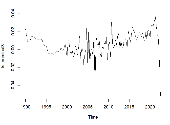
I used the log function because of the non-normality and took the first difference. After this, the real estate house prices were still not stationary, so I took the second difference which resulted in stationary data. The stock market data was stationary after taking the first difference, but I think I need to take the second difference as well in order to use it for the DCC-GARCH model.
The code I used for the DCC model is:
#perform DCC
model1=ugarchspec(mean.model = list(armaOrder=c(0,0)),variance.model = list(garchOrder=c(1,1),model="sGARCH"),distribution.model = "norm")
modelspec=dccspec(uspec = multispec(replicate(2,model1)),dccOrder = c(1,1), distribution = "mvnorm")
modelfit=dccfit(modelspec,data=(data.frame(ts_nominal,ts_share)))
modelfit
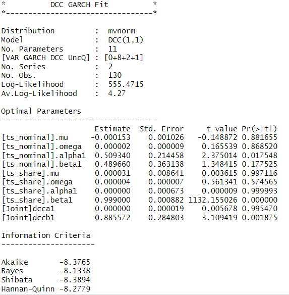
I'm not sure if I took the right steps to perform this analysis or if my code is even correct. Compared to other papers, I find it strange that only 3 parameters are significant and that alpha1 for stocks and dcca1 are almost equal to 1.
Can anyone help me with this?
Update: Further Research
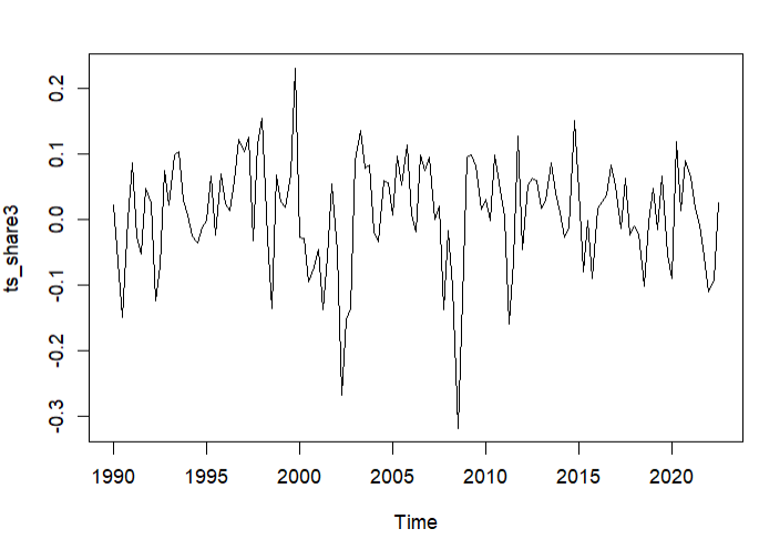
I have proceeded by taking the log return of both the property price index and stock price index. Then I used the diff() function, resulting in both time series being stationary. The results, however, are barely different than the last results I showed in the post.
Distribution         :  mvnorm
Model                :  DCC(1,1)
No. Parameters       :  11
[VAR GARCH DCC UncQ] : [0+8+2+1]
No. Series           :  2
No. Obs.             :  130
Log-Likelihood       :  502.7599
Av.Log-Likelihood    :  3.87

Optimal Parameters
-----------------------------------
                   Estimate  Std. Error     t value Pr(>|t|)
[ts_prop].mu       0.000547    0.003082    0.177488 0.859125
[ts_prop].omega    0.000011    0.000072    0.156417 0.875704
[ts_prop].alpha1   0.349696    0.649448    0.538451 0.590266
[ts_prop].beta1    0.649304    0.387195    1.676944 0.093553
[ts_share].mu      0.000031    0.008641    0.003615 0.997116
[ts_share].omega   0.000004    0.000007    0.561343 0.574564
[ts_share].alpha1  0.000000    0.000673    0.000009 0.999993
[ts_share].beta1   0.999000    0.000882 1132.157095 0.000000
[Joint]dcca1       0.000000    0.000007    0.000353 0.999719
[Joint]dccb1       0.895265    0.119982    7.461638 0.000000

Information Criteria
---------------------

Akaike       -7.5655
Bayes        -7.3229
Shibata      -7.5784
Hannan-Quinn -7.4669

Elapsed time : 0.909425
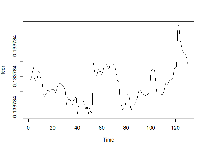
The next step in our analysis is to apply linear regression to see which determinants (like the long term interest rate) have a significant effect on the dynamic correlation between the property return time series and stock return time series. For this, I extracted the dynamic correlations from the DCC-GARCH model, but as you can see in the graph 'fcor', these correlations all have the same value of 0.133784 with minimal changes.
mod1=lm(fcor~long)
> summary(mod1)

Call:
lm(formula = fcor ~ long)

Residuals:
            Min              1Q          Median              3Q             Max
-0.000000010205 -0.000000003962 -0.000000001022  0.000000004495  0.000000019842

Coefficients:
                   Estimate      Std. Error       t value             Pr(>|t|)
(Intercept) 0.1337839573855 0.0000000005038 265555616.311 < 0.0000000000000002 ***
long        0.0000000045540 0.0000000016445         2.769              0.00646 **
---
Signif. codes:  0 ‘***’ 0.001 ‘**’ 0.01 ‘*’ 0.05 ‘.’ 0.1 ‘ ’ 1

Residual standard error: 0.000000005664 on 128 degrees of freedom
Multiple R-squared:  0.05652,   Adjusted R-squared:  0.04915
F-statistic: 7.669 on 1 and 128 DF,  p-value: 0.006455
I also performed regression on other determinants with all having a significant effect on the dynamic correlations. Can someone explain to me why the dynamic correlations barely change and why this has an effect on the linear regression result?

diff(log(...))with a single difference)? Also, what do you mean by variance test? Also, next time consider pasting the R output as text, not as picture. $\endgroup$diff(log(.))appears nonstationary, but it does not seem to have a unit root, and thus taking another difference is probably not an adequate measure. In this model, I would perhaps just use thediff(log(.))as is, even if it is nonstationary. But I do not have a solid defense of either choice. The problem is that the model is inadequate in either case due to the first series exhibiting some form of structural change. $\endgroup$