For this scenario, I would firstly ensure that you are in fact dealing with seasonal heteroscedasticity. This is a type of heteroscedasticity whereby variance of a time series increases at a particular time of year. For instance, variance in airline passenger numbers could see a significant increase during the summer months given higher passenger demand as compared to the winter. This reference might be of use: Is this seasonal heteroskedasticity?
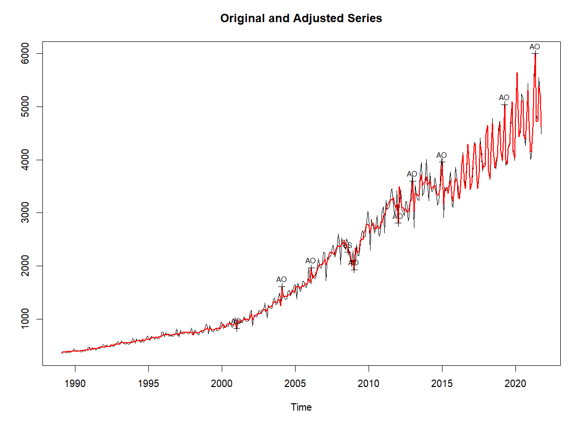
From analysing your time series, I am not sure whether seasonal heteroscedasticity is present per se - rather the variance in general is increasing across the time series which we typically see when analysing stock prices, for instance. This is known as conditional heteroscedasticity, whereby the variance of the error term at time t is dependent on that of t-1.
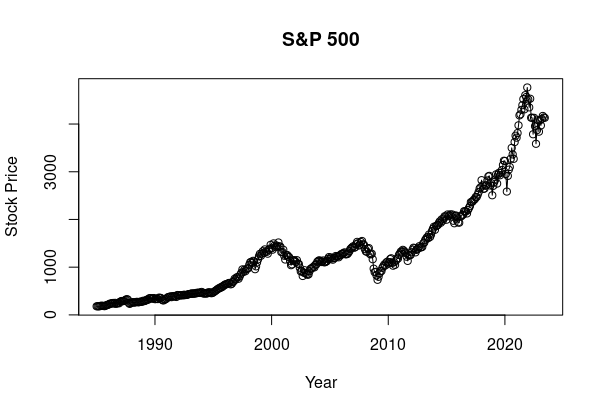
When analysing the S&P 500 for instance, we can see that the series shows greater swings in price for more recent years as compared to past years.

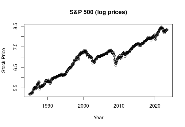
Using a logarithmic transformation, we see that the oscillations in price become more uniform as we are comparing the percentage differences in price over time as opposed to the raw price (this is a common transformation when dealing with financial data):

However, when testing for ARCH (autoregressive conditional heteroscedasticity effects) using archTest in R (available through the MTS library), we can see that a p-value of 0 is obtained when analysing the time series both with and without a log transformation. This indicates that the null hypothesis of no ARCH effects (p-value greater than 0.05) is rejected at the 5% level of significance, indicating that ARCH effects are present across the series.
> library(MTS)
> archTest(sp500_ts_log)
Q(m) of squared series(LM test):
Test statistic:  4234.925  p-value:  0
Rank-based Test:
Test statistic:  4227.456  p-value:  0

> library(MTS)
> archTest(sp500_ts)
Q(m) of squared series(LM test):
Test statistic:  3936.111  p-value:  0
Rank-based Test:
Test statistic:  4227.456  p-value:  0
In the above, we have seen that even with a log-transformation, ARCH effects remain as the variance in the error term remains inconstant due to time effects.
If the same test is run on a series of random numbers that are sampled from a normal distribution, we can see that the p-value is greater than 0.05, indicating that the null hypothesis of no ARCH effects cannot be rejected at the 5% level of significance.
> library(MTS)
> archTest(rnorm(1000))
Q(m) of squared series(LM test):
Test statistic:  10.7558  p-value:  0.3768576
Rank-based Test:
Test statistic:  5.230579  p-value:  0.8752523
Thus, for this particular scenario I would ensure that seasonal heteroscedasticity is in fact present in the model before attempting to correct for it. From eyeballing the graph, it appears as though conditional heteroscedasticity is present more generally. In addition, log-transforming the series would not be expected to remove the ARCH effects present across the time series.
