3
$\begingroup$

I have a simple dataset where I have fit y = 0 + x + I(x^2) for three altitude levels 1, 3, 6. I want to test whether the quadratic relationship is different for the three levels.

I can think of two ways of setting it up. But I need help with the interpretation

#1: A simple additive model
lm(y ~ 0 + x + I(x^2) + alt.level)

                   Estimate Std. Error t value Pr(>|t|)    
x                 7.684e+00  3.761e+00   2.043   0.0458 *  
I(x^2)           -7.292e-04  3.788e-04  -1.925   0.0594 .  
alt.level1        4.380e+03  7.350e+03   0.596   0.5537    
alt.level3        1.415e+04  6.617e+03   2.138   0.0370 *  
alt.level6        3.556e+04  6.617e+03   5.375 1.61e-06 ***


 #2: Interaction of the hump shape with each level
lm(y ~ 0 + x + I(x^2) * alt.level)
                                     Estimate Std. Error t value Pr(>|t|)    
x                                   7.769e+00  3.821e+00   2.033   0.0471 *  
I(x^2)                             -8.376e-04  4.319e-04  -1.940   0.0578 .  
alt.level1                          6.057e+03  8.056e+03   0.752   0.4555    
alt.level3                          1.287e+04  7.265e+03   1.772   0.0821 .  
alt.level6                          3.545e+04  7.265e+03   4.880 1.01e-05 ***
I(x^2):alt.level3                   1.530e-04  2.551e-04   0.600   0.5513    
I(x^2):alt.level6                  1.026e-04  2.551e-04   0.402   0.6892 


 #3: Interaction with the quadractic with hump shape
      lm(y ~ 0 + x + I(x^2) * alt.level)
       Coefficients:
                                     Estimate Std. Error t value Pr(>|t|)   
    x                               6.763e+00  7.068e+00   0.957  0.34313   
    I(x^2)                         -7.375e-04  7.302e-04  -1.010  0.31727   
    alt.level1                      6.782e+03  8.872e+03   0.764  0.44816   
    alt.level3                      2.081e+04  7.852e+03   2.650  0.01070 * 
    alt.level6                      2.696e+04  7.852e+03   3.433  0.00119 **
    x:alt.level3                   -9.593e+00  9.313e+00  -1.030  0.30781   
    x:alt.level6                    1.235e+01  9.313e+00   1.326  0.19085   
    I(x^2):alt.level3               1.082e-03  9.493e-04   1.140  0.25975   
    I(x^2):alt.level6             -1.098e-03  9.493e-04  -1.157  0.25262

I am not sure which is the right model to use for the question: Do the quadratic curves of each level significantly differ from the other? Also, I need some help with the interpretation of the output. For e.g. #3 is only asking if the linear term x alt.elvel1 is different from say the quadratic term of alt.level6 (last line of output). How can I ask if the curve in it's entirety is different between alt1 alt3 and alt6?

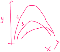
enter image description here

$\endgroup$
6
  • 1
    $\begingroup$ Based on your model, it appears you have removed the intercept. ¿Is there a theoretical reason to assume that the model ABSOLUTELY MUST pass thru the origin AND be a quadratic model? That is to say, ¿is there a reason the model would look like $y=ax(1+bx)$ instead of $y=a+bx+cx^2$? $\endgroup$
    – Gregg H
    Commented Jul 3, 2023 at 16:40
  • $\begingroup$ @GreggH Yes there is a biological reason for assuming it passes through origin and quadratic $\endgroup$ Commented Jul 3, 2023 at 16:58
  • 1
    $\begingroup$ Also, the outputs for #2 and #3 are different, but the way you typed the model is the same. $\endgroup$
    – Gregg H
    Commented Jul 3, 2023 at 17:10
  • 1
    $\begingroup$ Could you please edit the question to say something about what x represents biologically? I've been fooled by Mother Nature too often to rely on a strict theoretical form in modeling biological data. Sometimes it's better to fit a predictor like x more flexibly first and then document that the flexible fit is indistinguishable from the expected theoretical form. Knowing more about x would help in making that judgment or suggesting how to proceed with the quadratic modeling as you propose. $\endgroup$
    – EdM
    Commented Jul 3, 2023 at 17:33
  • 1
    $\begingroup$ Even when there is a theoretical region to pass through the origin, it's usually not a good idea to omit an intercept from the model. Frequently you will find that the intercept term is significant (and even large). That's valuable information that (a) could not be detected using a no-intercept model and (b) potentially shows that the coefficients for the no-intercept model might be (grossly) wrong. $\endgroup$
    – whuber
    Commented Jul 4, 2023 at 14:14

1 Answer 1

2
$\begingroup$

To model the different quadratic models for each level of the factor variable with the constraint that the models must always pass thru the origin $$y=ax + bx^2+\varepsilon,$$ you would need the following model

lm(y ~ -1 + x:alt.level + I(x^2):alt.level)

This will give you t-ratios and corresponding p-values to ask the following:

  • are the linear coefficients different from the reference group linear coefficient
  • are the quadratic coefficients different from the reference group quadratic coefficient

These are just the p-values you see in the coefficients output table. And the reference group is the one alt.level that is missing. Furthermore, the reference group coefficients would just be the x and I(x^2) parts of the table.

Note, if you are interested in where the maximum occurs (along the x-axis) or where the next intercept is, then the focus is probably going to be on the value of the quadratic coefficient (as the zero would be modeled to occur at $x_0 = -\frac{a}{b}$ and the extrema at half this value). But, if your focus is on the height of the zenith, then your focus will be on the linear coefficient (as this value omits the dependence on $b$, $y_o = -\frac{a^2}{4}$).

Happy to elaborate more if needed.

Edit #1
Sorry I missed the very last query...about comparing the models. If you wish to compare the model run with all the quadratic functions constrained to the same set of parameters (the same values for $a$ and $b$ mentioned above), then you can use this trick to run the model:

  1. Make sure you have dummy variables coded for each of your groups (I will call them d1 thru d3 here (or you can use the actual values in places of the number one in each dummy variable if the variable is actually ordinal or scalar...and not just categorical).
  2. Create the smaller model (with the constrained parameters. The trick for this is to create two new variables in the data frame: X=d1*x+d2*x+d3*x and Xsq=d1*xsq+d2*xsq+d3*xsq. Now, run this model as
    lm.const <- lm(y ~ -1 + X + Xsq)
    (This is the constrained model and can be thought of as model #1 or the smaller model for this comparison.)
  3. Now run the unconstrained model:
    lm.uncon <- lm(y ~ -1 + d1:x + d2:x + d3:x + d1:xsq + d2:xsq + d3:xsq)
    This is the full model (unconstrained) and can be called model #2 or the bigger model (as there are more parameters in the model).
  4. It may not appear that these models are nested, but they actually are (but you won't be able to use anova(·) to run the test. So, you will need to calculate the model comparison by hand. This is an F-ratio test with $F = \frac{R_2^1-R_1^2}{1-R_2^2} · \frac{df_{\text{err},2}}{4}$
    the 4 comes from the fact that there are 4 more parameters in the bigger model. This F-ratio follows an F-distribution with $df_n=4$ and $df_d=$df_{\text{err},2}$ degrees of freedom.

If the p-value for this F-ratio is less than your significance level, then you have different quadratic functions (in some manner or fashion) for the data. Else, the models are statistically equivalent, and use of the simpler (constrained) model is justified.

$\endgroup$
1
  • $\begingroup$ There would be 4 individual p values reported for the interaction between alt.level (with 3 levels) and the fit to x (with a linear and a quadratic term). To get at whether "the curve in it's entirety is different" among the altitudes, as the question asks, you would then need to do a combined Wald test on all those coefficients. It's possible for the overall fit to x to depend on alt.level even if none of the 4 coefficients is individually "significantly different" from 0, or vice-versa, depending on the covariances of the coefficient estimates. $\endgroup$
    – EdM
    Commented Jul 3, 2023 at 17:46

Your Answer

By clicking “Post Your Answer”, you agree to our terms of service and acknowledge you have read our privacy policy.

Not the answer you're looking for? Browse other questions tagged or ask your own question.