0
$\begingroup$

edit below

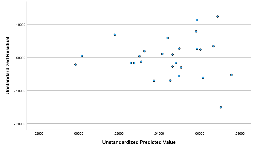
I am doing this analysis for the first time. How concerned should I be about heteroscedasticity in my data? Here's the scatterplot of predicted values vs residuals: scatterplot of predicted values vs residuals The Breusch-Pagan test is significant at p=.03 (χ²=4.682), so below <.05, but not .01.
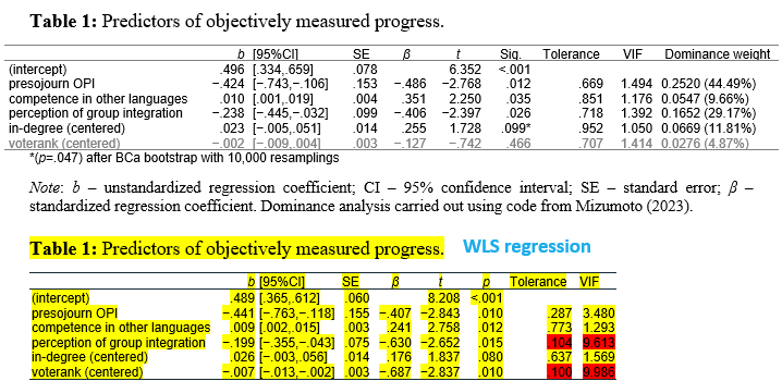
With regular multiple regression, the result is the first table below, quite nice. If instead I try WLS regression, the values change drastically (table highlighted in yellow), with two predictors ending up with unacceptable collinearity indices: enter image description here
Here is the original dataset if it helps: https://docs.google.com/spreadsheets/d/13U7xDK7otj-vBOcx6yTpsguAd-wlFNad/edit?usp=sharing&ouid=113244913961284427801&rtpof=true&sd=true

Thanks a lot in advance!

EDIT Thanks, Everyone, for the comments!

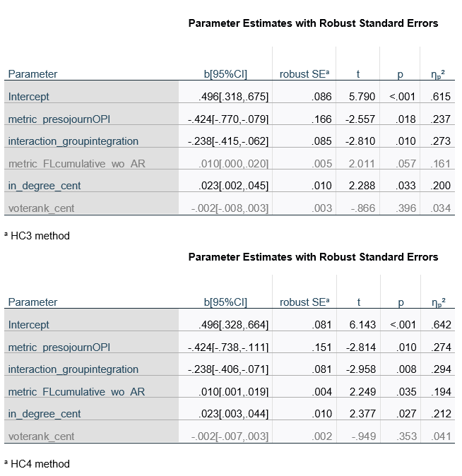
So, I ran regression with heteroscedasticity-consistent (robust) SEs:

regression with robust SEs

Is my understanding correct that the standardized beta values remain unchanged; what changes is the SEs, confidence intervals, p and t values, and effect sizes?

And, does anyone know how to get output for robust SEs complemented by i) confidence intervals for beta, ii) Tolerance and iii) VIF values (unless the latter two do not change with robust SEs; they do in weighted regression), either in SPSS or R?

$\endgroup$
2
  • 3
    $\begingroup$ A standard diagnostic plot suggests re-expressing your response variable in terms of its square root or possibly its logarithm. You have to proceed with great care here because you have very few data for the number of explanatory variables you employ. I notice, too, that you label Table 1 with "WLS regression." How did you determine the weights? $\endgroup$
    – whuber
    Commented Apr 2 at 13:32
  • $\begingroup$ @whuber: In our line of research (social network analysis reconstructing whole networks), we cannot just get more participants because we already have complete student cohorts; the best we can try to do is combine data from different years where we have them (not at the moment), but otherwise the studies will likely be underpowered. I can live with stating instability of the results in the limitations, but I do want to solve assumption violations first. To estimate weights I used the approach outlined in this video: youtube.com/watch?v=enPK_SXILnA $\endgroup$
    – mbp
    Commented Apr 6 at 14:54

1 Answer 1

3
$\begingroup$

There is heteroscedasticity, not only based on the Breusch–Pagan test, but also the very strong (more on that later) trend that can be seen in the residual plot (with increasing predicted value, the error is increasing as well).

The null hypothesis assumes homoskedasticity, this translates to the residuals staying relatively within the same range with increasing predicted value.

To quantify it better, I would say it is better to look at the standardized residual and check how many percentages the error is increasing. If you think that they are ok, then they are ok.

p=0.05 and p=0.01, are arbitrary in the sense that they are conventional thresholds rather than being determined by some universal law. If you choose to orient your statistics conservatively according to a 5% confidence level, then you have heteroscedasticity. If you choose a lenient approach with 1%, it seems like you don't, since the p that you got was at 3%.

I guess that you have some heteroscedasticity, but only if you test according to a 5% confidence level.

$\endgroup$
8
  • $\begingroup$ Thanks! Should I plot the standardized residuals against standardized predicted values, then, or still against unstandardized? Or feed the standardized residuals into an analysis? Isn't it the other way round, that I am dealing with heteroscedasticity if I assume alpha at .05 (as .03 is smaller) but not at .01? $\endgroup$
    – mbp
    Commented Apr 2 at 14:57
  • $\begingroup$ Plotting a normalized, e.g. range normalization to get something equivalent to a percentage, would suffice. No need to normalize predicted values. About the second point, you're right, I got my answer 180 degrees from the get-go, already corrected the first mistake and now you raised the second problem to my attention. I'll edit. $\endgroup$
    – Tino D
    Commented Apr 2 at 15:04
  • 1
    $\begingroup$ Overall this answer is good but it comes across I think as a bit equivocal. The diagnostic plot is text book heteroscedasticity. There are different schools of thought, but many people advocate against using tests of the assumptions of linear models and focusing on diagnostic plots. Transformations may help, but you may need a model that accounts for non-constant variance using generalized least squares $\endgroup$
    – N Brouwer
    Commented Apr 3 at 5:01
  • $\begingroup$ I agree that there is heteroscedasticity. And I also agree that there is room for improvement. However, the problem might not be as bad as it appears in the unstandardized residual plot since we do not know if an error of 0.1 in absolute value is important enough to care about. Transformation is a solution, or maybe using heteroskedasticity-consistent standard errors $\endgroup$
    – Tino D
    Commented Apr 3 at 10:24
  • $\begingroup$ @tino-d: Thanks! I ran the regression with HC SEs and updated the original question. I am happy with the output, especially for HC4, but a question here: Do you know how I can see the values for Tolerance and VIF for parameter estimates with "robust" SEs, either in SPSS or R? (Unless, like I assume betas, these do not change; they do in WLS.) $\endgroup$
    – mbp
    Commented Apr 6 at 15:00

Your Answer

By clicking “Post Your Answer”, you agree to our terms of service and acknowledge you have read our privacy policy.

Not the answer you're looking for? Browse other questions tagged or ask your own question.