How to obtain $p(x)$ given samples from $p(y|x)$ and $p(y)$?

Question

Here, assume both $p(y\mid x)$ and $p(y)$ are too complicated to get closed forms, and we can only draw samples from them. Is there any way to estimate or draw samples from $p(x)$?

Answer 1

This problem is equivalent to solving a Fredholm integral equation of the first kind. This is, solving for $p(x)$ such that:

$$ p(y) = \int_{\text{supp}(X)} p(y\mid x)\, p(x)\, \text{d}x,\quad \forall y\in \text{supp}(Y) $$

In general, this is an ill-posed inverse problem, and thus it is challenging for both analytical and numerical approaches. As @Glen_b mentions, a characterization of the support of $X$ is needed, as some approaches start off with its discretization.

For instance, notice that:

$$ p(x) = \int p(x\mid y)\,p(y)\,\text{d}y = \int \frac{p(y\mid x)\, p(x)}{\int p(y\mid \tilde{x})\, p(\tilde{x})\,\text{d}\tilde{x}}\,p(y)\,\text{d}y $$

This motivates a simple fixed-point iteration to solve for $p(x)$ in the case of $X$ being discrete with support $\{c_1,\cdots, c_d\}$, $d\geq 2$, and $p(y\mid x)$ being available for direct evaluation:

1. Initialize $p_0(x)=1/d$, $\forall x\in\{c_1,\cdots, c_d\}$
2. For each iteration step $n$, draw $m$ i.i.d. samples from $p(y)$, and let:

$$ p_{n}(x) = \frac{1}{m}\sum_{j=1}^m \frac{p(y_i\mid x)\, p_{n-1}(x)}{\sum_{i=1}^d p(y_j\mid c_i)\, p_{n-1}(c_i)},\quad \forall x\in\{c_1,\cdots, c_d\} $$

The motivation is that, for a sufficiently large $N$, $p_N(x)\approx p(x)$ in its support. This is based on:

Kondor (1983). Method of convergent weights — An iterative procedure for solving Fredholm's integral equations of the first kind. Nuclear Instruments and Methods in Physics Research, Volume 216, Issues 1–2, 1983, Pages 177-181, ISSN 0167-5087, https://doi.org/10.1016/0167-5087(83)90348-4.

There are more refined approaches including:

• Expectation Maximization Smoothing (EMS): Silverman et al (1990). A Smoothed EM Approach to Indirect Estimation Problems, with Particular, Reference to Stereology and Emission Tomography. Journal of the Royal Statistical Society. Series B (Methodological), 52(2), 271–324. http://www.jstor.org/stable/2345438
• Iterative Bayes (IB): Ma (2011). Indirect density estimation using the iterative Bayes algorithm. Computational Statistics & Data Analysis, Volume 55, Issue 3, 2011, Pages 1180-1195, ISSN 0167 9473, https://doi.org/10.1016/j.csda.2010.09.018.
• Sequential Monte Carlo (SMC): Crucinio et al (2023). A Particle Method for Solving Fredholm Equations of the First Kind. Journal of the American Statistical Association, 118(542), 937–947. https://doi.org/10.1080/01621459.2021.1962328

Answer 2

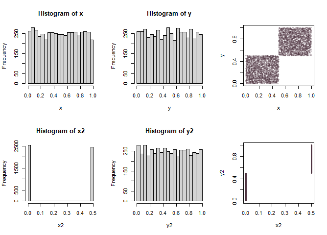
Depending on what we mean by specifying the conditional distribution, one possible answer is that we can't in general. If we specify the conditional distribution for $Y$, without specifying what the $X$ values are, we can get the same marginal distribution for $Y$ from different marginal distributions for $X$, for a given conditional distribution for $Y$.

Here's an example. (Other similar examples are possible. Whether this sort of example is particularly compelling is another story, because the particular form of conditional here "throws away" the information that distinguishes the $f(x)$'s. Xi'an's example in comments - which also does that but in a different manner - seems a little more satisfying, to be honest)

Let $f_{Y|X=x}(y) = 2$ $\text{ }I_{([2x]/2,([2x]+1)/2)}$, where $[\cdot]$ is the integer part of its argument.

Consider:

1. $X\sim \text{Bern}(\frac12)\text{ }\times\frac12$

2. $X\sim U(0,1)$

In both cases (and many others), $f_Y(y) = I_{(0,1)}$.

Here's the above simulated in R. The function ry.x randomly samples from the above conditional distribution given supplied x values; if we don't know the x's, we can't tell from that conditional and the resulting marginal for $Y$ what the $X$'s were.

ry.x = function(x) runif(length(x),floor(2*x)/2,floor(2*x+1)/2)
x = runif(5000)
y = ry.x(x)
x2 = rbinom(5000,1,.5)/2
y2 = ry.x(x2)
par(mfrow=c(2,3))
hist(x,n=50);hist(y,n=50);plot(x,y,pch=16,cex=.7,col=rgb(.3,.2,.25,.3))
hist(x2,n=50);hist(y2,n=50);plot(x2,y2,pch=16,cex=.7,col=rgb(.3,.2,.25,.3))