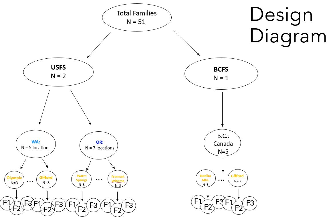
I have been trying to run a binomial GLMM on the proportion of emerged seedlings across locations (categorical variable) and over the monitoring period (continous variable). We obtained and planted seed from 3 distinct families within the same location, resulting in three proportions per location. The proportion is actually a "discrete proportion" where it is the number of emerged seedlings/the total number of seedlings grown for each family.
Therefore,my current model is:
M1A<-glmmTMB(Prob.emg ~ Location.parent.tree + Days.post.sowing + (1|Location.parent.tree/Fam.num), weights = Total.Seeds.Post.Harvest, family = binomial(link = "logit"), data = HM_M4)
Where:
- Location.parent.tree is the location name (e.g. Olympic National Park)
- Days.post.sowing is the number of days after sowing (e.g. 5, 10, 15...55 days)
- Fam.num is the family number
- Total.Seeds.Post.Harvest is the total number of seeds sown for each family. There are 51 families and 17 locations.
Here is a screenshot of the data and a figure of what the data design looks like:
The main point of the project is simply to say if the proportion of emerged seedlings differed between locations and if the proportion changed over time. The goal is to know which locations had the highest emergence abundance and which locations grew the fastest.
It recently was brought to my attention though that you cannot have the same variable as a fixed effect AND as a random effect via this other StackExchange question and via meeting with a statistician:
"If the grouping variable (a factor) is included as a covariate (Model fm2 below), both the random effects and its variance tend to be zero. The intuitive explanation is that, αi and ui basically model the same quantity (the group specific intercept), although one is assumed fixed and one is random. The majority of the variability is first absorbed by the fixed intercepts (αi), so the random intercepts ui tend to be all zero."
This issue shows up as a singular fit when I use check_singularity from the performance package and my RE variances are basically zero.
Family: binomial  ( logit )
Formula:
Prob.emg ~ Location.parent.tree + Days.post.sowing + (1 | Location.parent.tree/Fam.num)
Data: HM_M4
Weights: Total.Seeds.Post.Harvest

     AIC      BIC   logLik deviance df.resid
  3607.4   3684.8  -1783.7   3567.4      334

Random effects:

Conditional model:
 Groups                       Name        Variance  Std.Dev.
 Fam.num:Location.parent.tree (Intercept) 7.255e-01 8.517e-01
 Location.parent.tree         (Intercept) 2.567e-09 5.066e-05
Number of obs: 354, groups:  Fam.num:Location.parent.tree, 51; Location.parent.tree, 17

Conditional model:
                                             Estimate Std. Error z value Pr(>|z|)
(Intercept)                                 -3.137001   0.495709   -6.33 2.48e-10 ***
Location.parent.treeCrater Lake             -1.522821   0.701183   -2.17  0.02987 *
Location.parent.treeDeschutes               -0.643951   0.699187   -0.92  0.35705
Location.parent.treeFremont-Winema          -1.758760   0.705407   -2.49  0.01266 *
Location.parent.treeGifford Pinchot         -1.221386   0.703238   -1.74  0.08242 .
Location.parent.treeHoly Moly                0.449948   0.698670    0.64  0.51957
Location.parent.treeLime Mtn.                0.546800   0.698269    0.78  0.43358
Location.parent.treeMt. Hood                 0.210137   0.699067    0.30  0.76372
Location.parent.treeMtn Stevens             -0.440924   0.698507   -0.63  0.52789
Location.parent.treeNanika Mtn.              0.820801   0.698266    1.18  0.23980
Location.parent.treeNanika Mtn./Kid          1.241055   0.698446    1.78  0.07559 .
Location.parent.treeOkanogan-Wenatchee-East -1.376695   0.700487   -1.97  0.04937 *
Location.parent.treeOkanogan-Wenatchee-West -0.544422   0.698400   -0.78  0.43567
Location.parent.treeOlympic                 -1.860904   0.701079   -2.65  0.00795 **
Location.parent.treeUmpqua                  -1.961317   0.703158   -2.79  0.00528 **
Location.parent.treeWallowa-Whitman         -0.781231   0.700123   -1.12  0.26449
Location.parent.treeWarm Springs             0.891783   0.698564    1.28  0.20175
Days.post.sowing                             0.066089   0.001072   61.65  < 2e-16 ***
---
Signif. codes:  0 ‘***’ 0.001 ‘**’ 0.01 ‘*’ 0.05 ‘.’ 0.1 ‘ ’ 1
However, if I fit just the family number and don't have it nested within location, the model no longer has a singular fit (but the random effects structure is wrong).
While I have been told that your fixed effects should essentially be what you're interested in testing, I also know I repeatedly measured family proportions over time and that the families within locations are more likely to be similar to each other than other families in other locations (hence the nested random effect).
I now have some possible options to try to fix this, but it seems like I may not be able to get at my research question of how do the locations differ?
Option 1
M1B <- glmmTMB(Prob.emg ~ GPS.coord + Days.post.sowing + (1|Location.parent.tree/Fam.num), weights = Total.Seeds.Post.Harvest, family = binomial(link = "logit"), data = HM_M4)
The issue with this is that the GPS.coordinates are for each family (not representative of location), and I would somehow have to scale up the GPS coordinates for the 3 families to a higher "polygon" level?
Option 2
 > M1C <- glmmTMB(Prob.emg ~ Location.parent.tree + Days.post.sowing +
    > (1|Tray.num), weights = Total.Seeds.Post.Harvest, family =
    > binomial(link = "logit"), data = HM_M4)
Since each family was planted in a tray, I could use the tray number as a "dummy" variable for family number. I am not sure if this is "cheating" or not...
Option 3
Stick with what I have, knowing the RE isn't 100% accurate?
So my questions are:
Is it true that you can't use the same variable as an FE AND as an RE? I feel pretty against replacing location in the FE, since that's the main question of my project.
I have seen suggestions of running a fixed effects only model or a random effects only model to solve this issue. Is that true? Are there other options?
Thoughts on the possible models I listed? Would using tray number as a RE be allowed? Is there a way to manipulate GIS coordinates to a higher scale?


