Count data as an independent variable in OLS- using a dummy variable+ the variable linearly to account for skewness

Question

I am using OLS to model the relationship between amount of foreign aid (dependent variable, logged) and media coverage (number of newspaper articles, count variable). I assume a linear relationship between the two and use the "media coverage" variable as a continuous predictor. There is a spike in 0, however, in the count variable which makes it highly skewed to the right. Although this problem was addressed in different threads, I would like to better understand why using a dummy variable alongside the original variable would improve the model. What does the dummy variable do for the skewness? how can it be interpreted in parallel with the continuous part of the model? Moreover, do the values of 0 in the count variable have to be kept or replaced as "missing values" ?

I am also using a second IV, measuring the proportion of negative articles in the total amount of articles, which naturally spikes at the value of 0 as well. Does the dummy variable control for the zeros in this variable as well?

Thank you in advance!

Answer 1

In fact, including a dummy variable for when one of the explanatory variables is equal to zero will only improve the model if the reason there is a spike at zero also means your assumptions about the relationship between the variables are invalidated at that point. Otherwise you just have lots of variables with a common value for that explanatory variable, and there's nothing wrong with that.

Two common situations where the spike at zero does invalidate the assumed relationship are when zero really means either "unobserved" (true value was missed); or "truncated" (eg it really would have been a negative value if it could but can't go below zero). In your case for example, perhaps you are using media articles as a proxy for interest in a particular issue or country; your proxy measure can't go below zero, even though there may be differing degrees of lack of interest reflected by that variable.

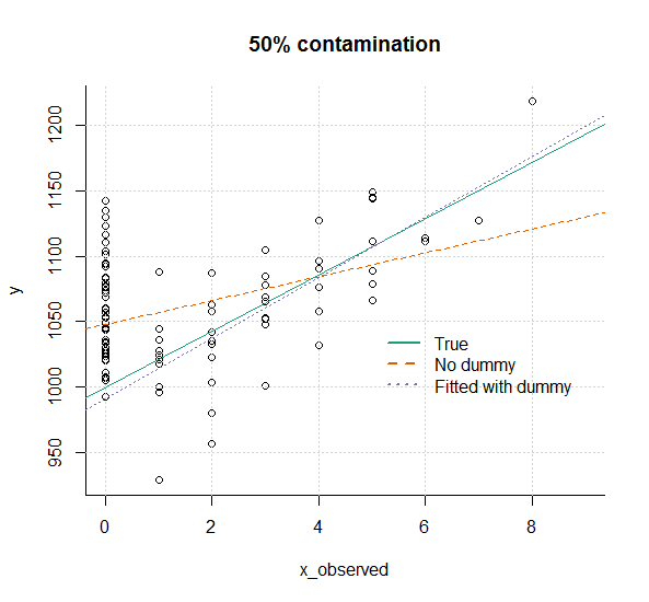
Consider the situation where in a certain number of cases zero really means the true value was not observed. In the plot below I generated data where there was a real, linear relationship between two variables, and then set 50% of the explanatory variables to zero to reflect a flawed observational process. You can see how if we just fit a linear model to the observed data the result is quite far from the true relationship of the underlying (partly unobserved data).

The principles are very similar when zero really stands in for a negative value but your observational process truncates it at zero (which might be your situation); except the bias in slope would be the other direction to that illustrated below.

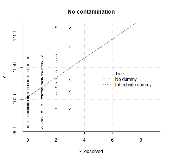
Conversely, imagine a case where the spike at zero is a natural result of the data generating mechanism. Adding a dummy makes no difference:

This would apply whether the large number of zeros is created by a nicely behaved distribution (as here, with Poisson(0.7) ) or were arbitrarily created - so long as they are set to zero before the response variable is generated based on its values.

(BTW why assume the relationship is linear? but that's another question).

Code in R that produced this is below.

demo_zero <- function(n=100, prob=.5, lam, ...){
  # demonstrate what happens when a proportion prob of an explanatory variable
  # is  wrongly observed as zero, independently of the generation of a 
  # response variable

  require(RColorBrewer)

  # Create a palette
  P <- brewer.pal(7, "Dark2")


  n <- 100

  # True data generating process
  x_true <- rpois(n, lam)
  y <- 1000 + 20 * x_true + rnorm(n,0,30)

  # Contaminate the Xs with some zeroes
  x_observed <- ifelse(runif(n) > prob, x_true, 0)

  # Create a dummy variable for when the observed x is zero
  dummy <- x_observed==0

  plot(x_observed, y, bty="l", xlim=c(0,9), ...)
  grid()
  abline(lm(y ~ x_true), lty=1, col=P[1])
  abline(lm(y ~ x_observed), lty=2, col=P[2])

  # will generate warning but is ok:
  abline(lm(y ~ x_observed + dummy), lty=3, col=P[3]) 

  legend(5,1050, c("True", "No dummy", "Fitted with dummy"), lty=1:3, col=P[1:3], bty="n", lwd=2)

}



demo_zero(prob=0.5, lam=3, main="50% contamination")

demo_zero(prob=.0, lam=.7, main="No contamination")