7
$\begingroup$

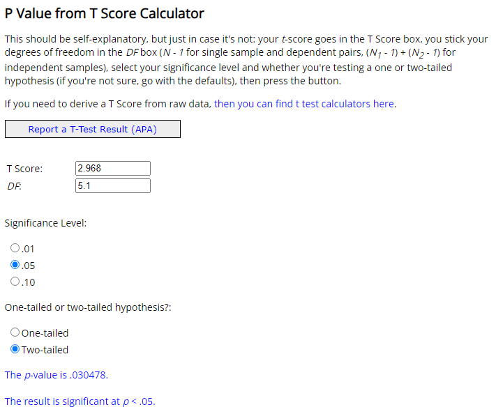
I am learning Welch's t-test and I successfully found that, in a two sample test, $t=2.968$ and the degree of freedom is $5.1$. I then go to an online p-value calculator for the p-value at 0.05 significance level. The results are as follows.

P value from Online Calculator

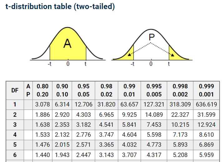
The problem is that I don't understand how the number $0.030478$ is generated. I tried to look at the two-tailed t-distribution table, but then I am not sure how to interpolate the p-value from the table. T table

Can anyone explain why $0.030478$ is the p-value here? Is it possible to get this number with the t-distribution table and a calculator only? I would like to learn how to get this number without the help of online calculator. Thanks in advance.

$\endgroup$

3 Answers 3

7
$\begingroup$

To get something out of the way first: you would not be calculating this by hand, pretty much ever. For certain integer degrees of freedom, the $t$ cumulative distribution function (CDF) reduces to something where this would be doable, but the general integral involves the Beta (or Gamma) function which you wouldn't be working out by hand, especially for non-integer values. We have a different kind of computer now than the ones that generated such tables.

That said, all of the functions you need for these calculations are defined for any positive degrees of freedom $\nu$. For example, the $t$ CDF can also be calculated in terms of the regularized incomplete Beta function $\text{B}$:

$$ P(T\le t) = \int_{-\infty}^tf(t)\ \text{d}t=\frac{1}{2}\ \text{B}\left(\frac{\nu}{t^2+\nu}, \frac{\nu}{2}, \frac{1}{2}\right). $$ This regularized incomplete Beta function is in reality just its CDF, so now you need to evaluate a Beta integral. Another alternative of the $t$ CDF includes evaluating an infinite sum. Some numerical approximations might be reasonable, though usually only in specific cases (e.g. large $\nu$). I hope that from all of this it's clear that attempting to tackle this problem to a high degree of precision using only pen and paper is an exercise in masochism.

Any statistical software package worth its salt will have implementations of these functions, for example the free & open-source R:

t <- 2.968
nu <- 5.1

## Calculate two-sided P-value directly:
2 * pt(-abs(t), nu)
#> 0.03047769

## One-sided lower tail via regularized Beta
oneside <- 0.5 * pbeta( nu/(nu+t^2), nu/2, 1/2)
## Two-sided
2 * oneside
#> 0.03047769

This bottom calculation is actually what pt does internally, albeit with a bit less care for numerical precision. Finally, a note of caution against interpolating from pre-calculated tables: for a given $t$-statistic the P-value is not a linear function of $\nu$.
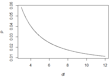
df vs. P-value

$\endgroup$
1
  • 1
    $\begingroup$ Thank you very much for your detailed explanation! I get a better understanding now! The mechanism behind these is indeed interesting. $\endgroup$
    – Am_2099
    Commented Oct 17 at 11:45
1
$\begingroup$

The accepted answer is good but I'll add an explanation of how to read the p-value table (with the caveat that you should really never need to do this, as mentioned in the accepted answer).

The guiding assumption for the table being presented in this way is that you don't actually care what your p-value is, just whether it is larger or smaller than some threshold (i.e., your significance level, so you can decide whether to reject your null hypothesis or not). Those significance levels are the columns and the degrees of freedom are the rows. Let's say your significance level was .05. Of course, 5.1 DF is not in the table, but 5 and 6 are, so the cutoff for the t-statistic is somewhere between 2.447 and 2.571 (closer to the latter). Your t-statistic is greater than both, thus your p-value is less than .05 and you would reject the null hypothesis.

If instead your significance level (as set a priori) was .02, then you would only reject the null if your t-statistic was higher than some number between 3.143 and 3.365 (again, closer to the latter). In this case your observed t-statistic is lower than both, so the p-value must be larger than .02.

As your online calculator (or some R code) points out, the p-value is ~.03, which of course is larger than .02 and smaller than .05. But you would have no way of knowing it is precisely 0.030478... from the table. And with decimal degrees of freedom, these tables become effectively useless--for example, what if your significance level was .02 and your observed t-statistic was 3.25? You wouldn't be able to tell whether to reject or not.

$\endgroup$
1
$\begingroup$

Besides statistical programs such as R being able to calculate this directly for you, you can get most spreadsheets to do this calculation.

However, if you do happen to be stuck with just a calculator and a table for some reason, see How do I find values not given in statistical tables?. In this case you'd be interpolating in both tail probability and degrees of freedom. In a case like this where you're dealing with small d.f. and tail areas somewhere in the region of 5%, I'd suggest linear interpolation in log of tail area and leaving d.f. as is as sufficient while still pretty accurate.

Since we have 5.1 d.f., we focus on rows for 5 and 6 d.f. and since the value is around 2.9 we need the p-values for 0.05 and 0.02.

In this circumstance, interpolation in d.f. to get approximate 5% and 2% values for 5.1 d.f, and then interpolating in $\log(p)$ using the observed t-statistic would be an easy way to proceed.

Dealing with the fractional d.f. first. We want to go 10% of the way from 5 d.f. toward 6 d.f.

Following the methodology discussed at the link with linear interpolation in d.f., this gives a 5% critical value of 2.5586 (keeping an additional figure for intermediate calculation to avoid impact from premature rounding), and a 2% critical value of 3.3428 (note that these are only accurate to roughly 3 significant figures). Then applying linear interpolation of the log of the p-value, using the observed t-value of 2.968 between these critical values, we get a $\log(p)$ of about -3.474 and so a p-value of about 0.031 when the "exact" value comes out to 0.0305 (which is itself an approximation, since Welch-statistics are not actually t-distributed).

This is not too bad an approximation when working from tables. Greater accuracy is possible but usually not worth additional effort. There would be few instances where you'd ever want to do this, though.

$\endgroup$

Your Answer

By clicking “Post Your Answer”, you agree to our terms of service and acknowledge you have read our privacy policy.

Not the answer you're looking for? Browse other questions tagged or ask your own question.