Mixture of non-normals is normal?

Question

Does anyone have a simple example of a mixture of non-normal distributions that is normal? To make life simple, pick specific $f_1(y)$ and $f_2(y)$, both with mean 0, such that $$(1/2)f_1(y) + (1/2)f_2(y) = \frac{\exp(-y^2/2)}{\sqrt{2\pi}}.$$

Such distributions would provide a neat counterexample to the commonly stated "fact" that normality of the regression residuals implies normality of the conditional distributions. Let $Y|X = 1 \sim f_1(y)$ and $Y|X =2 \sim f_2(y)$. Further, let $X$ take the values 1 and 2 each with probability 1/2. Then the marginal distribution of the true residuals is normal, while the conditional distributions of $Y$ are not.

(Comment: It is the marginal distribution of the residuals that is most often used to check the normality assumption.)

Answer 1

I can show you all examples, not just the simple ones.

Solution

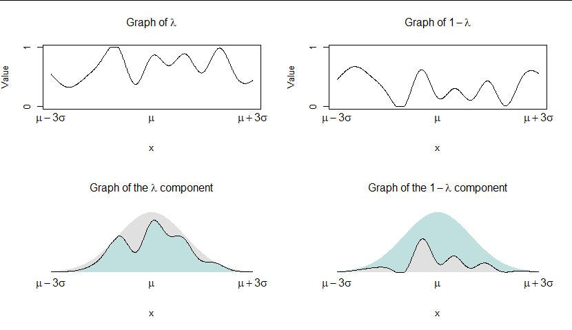
Here they are, schematically:

The bottom panels show how the density function $f$ of a distribution $F$ is split into two parts vertically along a nearly arbitrary curve. The cyan portion of the split is a fraction $\lambda$ of $f;$ the upper left plots its graph. The remaining portion (gray) therefore is a fraction $1-\lambda$ of $f$ whose graph is plotted in the upper right. This is how all mixtures arise.

(Notice that little is assumed about the density $f$ except that it exists.)

---

Details

The mixture distribution $F$ is Normal, which means there is a mean $\mu$ and variance $\sigma^2$ for which $F$ has a density function $f(z;\mu,\sigma).$ The details of $f$ don't matter!

Let $\lambda:\mathbb{R}\to[0,1]$ be any (measurable) non-negative function. This means the following integrals involving $\lambda$ are defined and non-negative:

$$\pi_\lambda = \int_\mathbb{R} \lambda(z)f(z;\mu,\sigma)\,\mathrm{d}z \le \sup(\lambda)\, \int_\mathbb{R}f(z;\mu,\sigma)\,\mathrm{d}z \le (1)(1)=1;$$

$$1-\pi_\lambda = 1 - \int_\mathbb{R} \lambda(z)f(z;\mu,\sigma)\,\mathrm{d}z = \int_\mathbb{R} (1-\lambda(z))_f(z;\mu,\sigma)\,\mathrm{d}z \le 1.$$

(The first inequality is an easy special case of Holder's Inequality.)

Define two distributions as

$$F_{\lambda}(x) = \frac{1}{\pi_\lambda}\int_{-\infty}^x \lambda(z)f(z;\mu,\sigma)\,\mathrm{d}z;$$

$$F_{1-\lambda}(x) = \frac{1}{1-\pi_\lambda}\int_{-\infty}^x (1-\lambda(z))f(z;\mu,\sigma)\,\mathrm{d}z.$$

It is straightforward to establish that these are distribution functions and, by construction,

$$F = \pi_\lambda F_\lambda + (1-\pi_\lambda) F_{1-\lambda}\tag{*}$$

exhibits the original normal distribution as a mixture of these two.

Conversely, whenever there exist differentiable functions with property $(*),$ then a version of $\lambda$ can be recovered via

$$\lambda(z) = \left\{\begin{aligned}\frac{F^\prime_\lambda(z)}{f(z;\mu,\sigma)} &\quad&f(z;\mu,\sigma)\ne 0\\ 0 & &\text{otherwise}\end{aligned}\right.$$

and because $0 \le \pi_\lambda\le 1,$ the range of $\lambda$ is contained in $[0,1],$ QED.

Finally, it is possible for the component distributions to be Normal: for instance, when $\lambda$ is a constant function that will be the case. That is the only possibility, though: see https://stats.stackexchange.com/a/429877/919 for the proof.

---

Application

As requested in comments, it would be of interest to choose $\lambda$ to meet a set of criteria, such as

1. Give the components equal weights, which means $$\frac{1}{2}=\pi_\lambda = \int \lambda(z) f(z)\,\mathrm{d}z.$$

2. Since these are intended to model errors in a regression setting (with $\mu=0,$ we would like each of the components also to have zero mean: $0 = E_{F_\lambda}[X].$ In light of (1), that is equivalent to $$0 = \int z\lambda(z) f(z)\,\mathrm{d}z.$$

3. Since regression errors are often assumed to be homoscedastic -- of equal variances -- we would like the variances of $F_\lambda$ and $F_{1-\lambda}$ to be equal. Since they have means of zero, when $f$ is a Normal density, this is achieved when $$\sigma^2 = 2\int z^2\lambda(z) f(z)\,\mathrm{d}z.$$

Although there are many solutions to these equations, one simple (striking) solution is obtained by supposing $\lambda$ and $1-\lambda$ are both simple functions: that is, piecewise constant. By making $\lambda$ symmetric around $0$ we can assure that (2) holds. The simplest of such simple functions is zero except on some positive interval $[a,b]$ and its negative $[-b,-a],$ where it equals $1.$

Without any loss of generality take $\sigma^2=1,$ so that $f = \phi$ is the standard Normal density with the property $\phi^(z) = -z\phi(z).$ Using this fact we may compute

$$\int \lambda(z)\phi(z)\,\mathrm{d}z = 2 \int_a^b \phi(z)\,\mathrm{d}z = 2(\Phi(b)-\Phi(a))$$

(where $\Phi$ is the standard Normal distribution function) and

$$\begin{aligned} \int z^2 \lambda(z)\phi(z)\,\mathrm{d}z &= 2 \int_a^b z^2\phi(z)\,\mathrm{d}z \\ &= 2(\Phi(b) - \Phi(a) + a\phi(b) - b\phi(b)). \end{aligned}$$

This permits numerical solution of (1) and (3). The work is streamlined by noting from (1) that, given $0 \le a\lt \Phi^{-1}(3/4),$

$$b = b(a) = \Phi^{-1}(\Phi(a) + 1/4).$$

That leaves us to solve (3) for $a \ge 0$. Here is an R implementation to illustrate:

f <- function(a) {
  b <- qnorm(1/4 + q <- pnorm(a))
  pnorm(b) - q + a * dnorm(a) - b * dnorm(b) - 1/4
}
uniroot(f, c(0, qnorm(3/4)- 1e-6))$root -> a
qnorm(pnorm(a) + 1/4) -> b

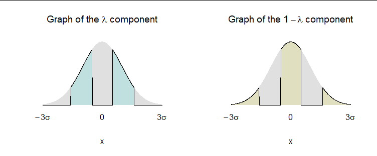
This calculation gives $a \approx 0.508949$ and $b \approx 1.59466.$ Here are plots of the two component densities $f_\lambda$ and $f_{1-\lambda}:$

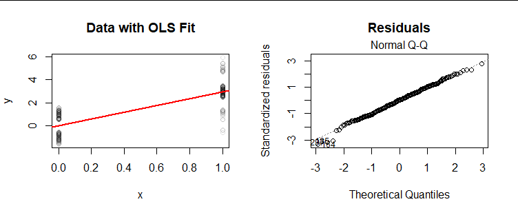
To illustrate the intended application, here are bivariate data with 150 responses at $X=0$ with errors distributed as $F_\lambda$ and 150 responses at $X=1$ with errors distributed as $F_{1-\lambda}.$ To the right is a quantile plot of the collected residuals.

Although separately neither group of residuals appears Normal, they are both centered at zero, have nearly the same variance, and collectively look perfectly Normal.

---

Remarks

1. The basic construction readily generalizes to mixtures with more than two components.

2. The example in the application can be extended, by using simple (indicator) functions supported on intervals $[a_i,b_i]$ with $0\le a_1 \lt b_1 \le a_2 \lt b_2 \cdots \lt b_k,$ to create component distributions that match the first $2k$ moments of the Normal distribution their mixture creates. With sufficiently large $k,$ the component distributions will be difficult to discriminate even with largish datasets (at which point one might legitimately wonder whether their non-Normality matters at all).

Answer 2

A very simple example from the Skew normal distribution with density $$ 2\phi(x)\Phi(\alpha x) $$ Choose for the twocomponents $\alpha, -\alpha$ then $$ \frac12 2 \phi(x) \Phi(-\alpha x) + \frac12 2 \phi(x) \Phi(\alpha x) $$ is the standard normal density $\phi(x)$, by using symmetry, since $\Phi(-\alpha x) = 1-\Phi(\alpha x)$, but unfortunately the two mixture components do not have equal mean.

A simple example with equal means is got by exploiting $1=\sin^2 x +\cos^2 x$ so simply define mixture components by $$ \phi(x) = \sin^2(x) \phi(x) + \cos^2(x) \phi(x) $$ and both components have mean zero.