There is a relatively simple resolution of this problem: compute a “fiducial limit” based on “inverse regression” [Draper & Smith 1981]. The idea is to create confidence envelopes for the true line and then find the range of $X$ values where these envelopes enclose the target response.
After introducing some notation (intended to match that in Draper & Smith), this answer performs a preliminary analysis of the situation, illustrates the idea with a plot of simulated data, and presents the formulas. It concludes with a brief discussion (in which a simple approximation is presented) and a reference to the principal source of this solution, Draper & Smith's regression textbook.
(The source of this answer is a report I wrote years ago concerning ongoing monitoring of concentrations in the environment: the $X_i$ were time and the $Y_i$ were log concentrations. The problems of (a) monitoring to determine when a value will reach a predetermined target and (b) calibration of measurement systems--where the $X_i$ are known values and the $Y_i$ are the instrument's responses--are the two situations in which I have found this procedure to be most useful.)
Let's establish notation. The data are $(X_i, Y_i)$, $i=1, 2, \ldots, n$. The model is
$$Y_i = \beta_0 + \beta_1 X_i + \varepsilon_i$$
for unknown parameters $\beta_0$ (the intercept) and $\beta_1$ (the slope) and independent Normal, zero-mean variates $\varepsilon_i$ with common (unknown) variance $\sigma^2$. Ordinary Least Squares regression obtains estimates $b_0$, $b_1$, and $s$ of the unknowns $\beta_0$, $\beta_1$, and $\sigma$. The calculations that enter into those estimates include the means $\bar X$ and $\bar Y$ as well as the sum of squared deviations of the $X_i$,
$$S_{XX} = \sum_{i=1}^n (X_i - \bar{X})^2.$$
Analysis
To begin the analysis, note that the regression line necessarily passes through the point of averages $(\bar{X}, \bar{Y})$, signifying an average response $\bar Y$ attained at the average ordinate $\bar X$. Moreover, the abscissa $\bar Y$ is Normally distributed, uncorrelated with the estimated slope $b_1$, and has a standard error that decreases to zero as the amount of data increases. The value of $X$ for any given $Y_0$ can be estimated by starting here and extrapolating, yielding an estimate of
$$\hat{X}_0 = (\bar{Y} - Y_0)/b_1 + \bar X.$$
The second step is to note that for any value $X$ we can compute an upper confidence limit for the fitted response at $X$. The need for a confidence limit arises from uncertainty about the values of the coefficients $\beta_0$ and $\beta_1$: we are not exactly sure of the true intercept and true slope, so the true line really could lie within a range of possible lines. The fitted response at $X$ can be written
$$\hat{Y}(X) = \bar{Y} - b_1(X - \bar{X})$$
and the standard error of that fitted value equals
$$\operatorname{se}(\hat{Y}(X)) = s\left(\frac{1}{n} + \frac{(X - \bar{X})^2}{S_{XX}}\right)^{1/2}.$$
The fitted value is Normally distributed, whence an upper confidence limit of confidence $1 - \alpha$ can be constructed of the form
$$\operatorname{UCL}(X) = \hat{Y}(X) + t(n-2, \alpha) \operatorname{se}(\hat{Y}(X))$$
and a lower confidence limit (LCL) is constructed analogously. (As usual, $t$ refers to percentage points of a Student $t$ distribution.) As $X$ varies, the UCL and LCL trace hyperbolic arcs lying above and below the fitted line.

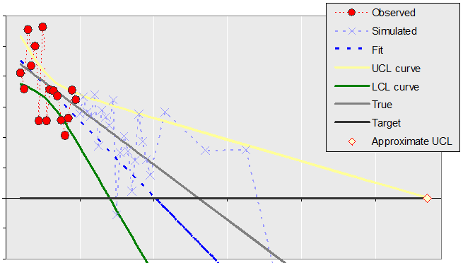
The horizontal axis plots the $X$ values while the vertical axis plots the $Y$ values. The hyperbolic arcs are shown as green (LCL) and yellow (UCL) curves. The fiducial limits are found by intersecting these arcs with a horizontal line at the height $Y_0\,$ designated "Target" in the legend. The resulting UCL is shown with a diamond symbol. This illustration uses simulated data: this allows us to see how additional data might reasonably vary from what the calculations lead us to expect. (The reason why "observed" and "simulated" values have been visually connected is that this shows a plot of concentration vs. time of a presumably continuous process.)
Solution
To find the “upper fiducial limit,” or “inverse confidence limit for $X$ given $Y_0$” ([Draper & Smith 1981] section 1.7), find the largest solution $X$ of the equation
$$Y_0 = \operatorname{UCL}(X),$$
if such a solution exists. This can be solved with the quadratic formula, giving
$$\operatorname{UCL}(X) = \bar{X} + \frac{D_0 + g\sqrt{D_0^2 + (1-g^2)S_{XX}/n}}{1-g^2}, \tag{1}$$
where
$$D_0 = (\bar Y - Y_0) / b_1$$
is the estimated value of $X$ corresponding to $Y_0$,
$$g^2 = \frac{t^2 s^2}{b_1^2 S_{XX}}$$
is an auxiliary calculation, and
$$t = t(n-2, \alpha).$$
A lower confidence limit on $X$ is obtained by using the negative square root $–g$ in $(1)$. (These formulas are equivalent to [Draper & Smith] equation 1.7.6. I write $g^2$ here in place of their $g$. This version is a little easier to compute with.)
Discussion
Neither confidence limit has to exist. They can be found only when there is confidence that the slope truly is nonzero. Draper & Smith suggest that computing confidence limits for $X$ is “not of much practical value” unless $g^2 < 0.2$, although they do not provide any justification for such an omnibus statement.
When $g^2$ is relatively small, a good approximation is obtained by expanding $(1)$ in a power series in its positive square root $g$ and stopping after the linear term, yielding
$$\operatorname{UCL}(X) \approx \bar{X} + D_0 + g\sqrt{D_0^2 + S_{XX}/n} + \cdots\tag{2}.$$
Note that $g^2$ is small when, relative to the estimated variance $s^2$, the estimated coefficient $b_1$ is large, the variance of the $X_i$ (that is, $S_{XX}/n$) is large, and $t$ is small (that is, extremely high confidence is not required). In short, any combination of a large absolute slope, wide spread in the $X_i$, large amounts of data, relatively small variation around a linear curve, and/or modest confidence needs will assure the approximation $(2)$ is a good one. Also note that as additional data are collected throughout a range of $X$ values that cover the confidence limit, $\operatorname{UCL}(X)$ converges to $\bar{X}+D_0$ , the estimated value, as one would expect of a genuine confidence limit.
References
Draper, NR and H Smith, 1981: Applied Regression Analysis, Second Edition. John Wiley & Sons, New York.


