47
$\begingroup$

For a unimodal distribution that is moderately skewed, we have the following empirical relationship between the mean, median and mode: $$ \text{(Mean - Mode)}\sim 3\,\text{(Mean - Median)} $$ How was this relationship derived?

Did Karl Pearson plot thousands of these relationships before forming this conclusion, or is there a logical line of reasoning behind this relationship?

$\endgroup$

3 Answers 3

34
$\begingroup$

Denote $\mu$ the mean ($\neq$ average), $m$ the median, $\sigma$ the standard deviation and $M$ the mode. Finally, let $X$ be the sample, a realization of a continuous unimodal distribution $F$ for which the first two moments exist.

It's well known that

$$|\mu-m|\leq\sigma\label{d}\tag{1}$$

This is a frequent textbook exercise:

\begin{eqnarray} |\mu-m| &=& |E(X-m)| \\ &\leq& E|X-m| \\ &\leq& E|X-\mu| \\ &=& E\sqrt{(X-\mu)^2} \\ &\leq& \sqrt{E(X-\mu)^2} \\ &=& \sigma \end{eqnarray} The first equality derives from the definition of the mean, the third comes about because the median is the unique minimiser (among all $c$'s) of $E|X-c|$ and the fourth from Jensen's inequality (i.e. the definition of a convex function). Actually, this inequality can be made tighter. In fact, for any $F$, satisfying the conditions above, it can be shown [3] that

$$|m-\mu|\leq \sqrt{0.6}\sigma\label{f}\tag{2}$$

Even though it is in general not true (Abadir, 2005) that any unimodal distribution must satisfy either one of $$M\leq m\leq\mu\textit{ or }M\geq m\geq \mu$$ it can still be shown that the inequality

$$|\mu-M|\leq\sqrt{3}\sigma\label{e}\tag{3}$$

holds for any unimodal, square integrable distribution (regardless of skew). This is proven formally in Johnson and Rogers (1951) though the proof depends on many auxiliary lemmas that are hard to fit here. Go see the original paper.


A sufficient condition for a distribution $F$ to satisfy $\mu\leq m\leq M$ is given in [2]. If $F$:

$$F(m−x)+F(m+x)\geq 1 \text{ for all }x\label{g}\tag{4}$$

then $\mu\leq m\leq M$. Furthermore, if $\mu\neq m$, then the inequality is strict. The Pearson Type I to XII distributions are one example of family of distributions satisfying $(4)$ [4] (for example, the Weibull is one common distribution for which $(4)$ does not hold, see [5]).

Now assuming that $(4)$ holds strictly and w.l.o.g. that $\sigma=1$, we have that $$3(m-\mu)\in(0,3\sqrt{0.6}] \mbox{ and } M-\mu\in(m-\mu,\sqrt{3}]$$

and since the second of these two ranges is not empty, it's certainly possible to find distributions for which the assertion is true (e.g. when $0<m-\mu<\frac{\sqrt{3}}{3}<\sigma=1$) for some range of values of the distribution's parameters but it is not true for all distributions and not even for all distributions satisfying $(4)$.

  • [0]: The Moment Problem for Unimodal Distributions. N. L. Johnson and C. A. Rogers. The Annals of Mathematical Statistics, Vol. 22, No. 3 (Sep., 1951), pp. 433-439
  • [1]: The Mean-Median-Mode Inequality: Counterexamples Karim M. Abadir Econometric Theory, Vol. 21, No. 2 (Apr., 2005), pp. 477-482
  • [2]: W. R. van Zwet, Mean, median, mode II, Statist. Neerlandica, 33 (1979), pp. 1--5.
  • [3]: The Mean, Median, and Mode of Unimodal Distributions:A Characterization. S. Basu and A. DasGupta (1997). Theory Probab. Appl., 41(2), 210–223.
  • [4]: Some Remarks On The Mean, Median, Mode And Skewness. Michikazu Sato. Australian Journal of Statistics. Volume 39, Issue 2, pages 219–224, June 1997
  • [5]: P. T. von Hippel (2005). Mean, Median, and Skew: Correcting a Textbook Rule. Journal of Statistics Education Volume 13, Number 2.
$\endgroup$
10
  • $\begingroup$ I am sorry, I am just a first year math student. Could you please provide/recommend a link/book/paper that describes how the relationship was derived? $\endgroup$
    – Sara
    Commented Oct 20, 2010 at 8:52
  • 3
    $\begingroup$ @Sara I think it dates back to Karl Pearson, which uses this empirical relationship for his "Pearson mode skewness". Aside from this, you may find interesting this online article, j.mp/aWymCv. $\endgroup$
    – chl
    Commented Oct 20, 2010 at 9:42
  • $\begingroup$ If mean is unique minimizer, shouldn't it be $E|X-\mu|\le E|X-m|$? $\endgroup$
    – mpiktas
    Commented Dec 9, 2010 at 13:09
  • 2
    $\begingroup$ Various points: $E|X-k|$ is minimised when $k$ is the median of $X$. Von Hippel's article (linked above by chl) discuses exceptions and btinternet.com/~se16/hgb/median.htm shows the possible relationship between mean, median, mode and standard deviation, both for continuous and for discrete distributions. The 3 can in fact take any value: positive, negative, zero or infinite. $\endgroup$
    – Henry
    Commented Feb 9, 2011 at 8:18
  • 1
    $\begingroup$ It may be that I am being a little dense (it wouldn't be the first time). Can you clarify how $|M-\mu|\leq 3|\mu-m|$ follows from (1) and (3)? $\endgroup$
    – Glen_b
    Commented Feb 1, 2015 at 12:06
9
$\begingroup$

The paper chl points to gives some important information -- showing that it's not close to a general rule (even for continuous, smooth, "nicely behaved" variables, like the Weibull). So while it may often be approximately true, it's frequently not.

So where is Pearson coming from? How did he arrive at this approximation?

Fortunately, Pearson pretty much tells us the answer himself.

The first use of the term "skew" in the sense we're using it seems to be Pearson, 1895 [1] (it appears right in the title). This paper also appears to be where he introduces the term mode (footnote, p345):

I have found it convenient to use the term mode for the abscissa corresponding to the ordinate of maximum frequency. The the "mean," the "mode," and the "median" have all distinct characters important to the statistician.

It also appears to be his first real detailing of of his system of frequency curves.

So in discussing estimation of the shape parameter in the Pearson Type III distribution (what we'd now call a shifted - and possibly flipped - gamma), he says (p375):

The mean, the median, and the mode or maximum-ordinate are marked by bb, cc and aa, respectively, and as soon as the curves were drawn, a remarkable relation manifested itself between the position of the three quantities: the median, so long as $p$ was positive* was seen to be about one-third from the mean towards the maximum$^\dagger$

* this corresponds to the gamma having shape parameter $>1$

$\dagger$ here the intent of "maximum" is the $x$-value of the maximum frequency (the mode), as is clear from the beginning of the quote, not the maximum of the random variable.

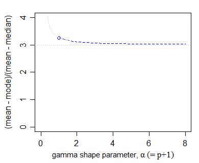
And indeed, if we look at the ratio of (mean-mode) to (mean-median) for the gamma distribution, we observe this:
enter image description here

(The blue part marks the region Pearson says that the approximation is reasonable).

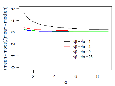
Indeed, if we look at some other distributions in the Pearson system - say the beta distributions, for example - the same ratio approximately holds as long as $\alpha$ and $\beta$ are not too small:
enter image description here

(the particular choice of subfamilies of the beta with $\sqrt{\beta}-\sqrt{\alpha}=k$ was taken because of the appearance of $\sqrt{\beta}-\sqrt{\alpha}$ in the moment skewness, in such a way that increasing $\alpha$ for constant $\sqrt{\beta}-\sqrt{\alpha}$ corresponds to decreasing moment skewness. Interestingly, for values of $\alpha$ and $\beta$ such that $\sqrt{\beta}+\sqrt{\alpha}=c$, the curves have almost constant (mean-mode)/(mean-median), which suggests that we might be able to say that the approximation is reasonable if $\sqrt{\beta}+\sqrt{\alpha}$ is large enough, though possibly with some minimum on the smaller of $\alpha$ and $\beta$.)

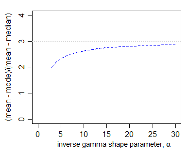
The inverse gamma is also in the Pearson system; it, too, has the relationship for large values of the shape parameter (say roughly $\alpha>10$):
enter image description here

It should be expected that Pearson was also familiar with the lognormal distribution. In that case the mode, median and mean are respectively $e^{\mu-\sigma^2}, e^{\mu}$ and $e^{\mu+\sigma^2/2}$; it was discussed prior to the development of his system and is often associated with Galton.

Let us again look at (mean-mode)/(mean-median). Cancelling out a factor of $e^{\mu}$ from both numerator and denominator, we're left with $\frac{e^{\sigma^2/2}-e^{-\sigma^2}}{e^{\sigma^2/2}-1}$. To first order (which will be accurate when $\sigma^2$ is small), the numerator will be $\frac{3}{2}\sigma^2$ and the denominator $\frac{1}{2}\sigma^2$, so at least for small $\sigma^2$ it should also hold for the lognormal.

There are a fair number of well known distributions - several of which Pearson was familiar with - for which it is close to true for a wide range of parameter values; he noticed it with the gamma distribution, but would have had the idea confirmed when he came to look at several other distributions he'd be likely to consider.

[1]: Pearson, K. (1895),
"Contributions to the Mathematical Theory of Evolution, II: Skew Variation in Homogeneous Material,"
Philosophical Transactions of the Royal Society, Series A, 186, 343-414
[Out of copyright. Freely available here]

$\endgroup$
6
$\begingroup$

This relationship was not derived. It was noticed to approximately hold on near symmetric distributions empirically. See Yule's exposition in The Introduction to the theory of statistics, (1922), p.121, Chapter VII Section 20. He presents the empirical example.

$\endgroup$
3
  • 1
    $\begingroup$ +1 Indeed, my quote of Pearson 1895 indicates that it's something he noticed rather than derived. $\endgroup$
    – Glen_b
    Commented Oct 29, 2015 at 1:02
  • 2
    $\begingroup$ Old math texts are so much more fun to read than today's writing $\endgroup$
    – Aksakal
    Commented Oct 29, 2015 at 1:06
  • 1
    $\begingroup$ Not that it really matters, but when I did some research on the book (because I want to cite it) I found that the relation was already pointed out in the first edition of the book published in 1911. $\endgroup$
    – mapf
    Commented Aug 19, 2020 at 7:37

Not the answer you're looking for? Browse other questions tagged or ask your own question.