Irregular time series with multiple sampling sites

Question

I have a dataset of marine debris items (number of items standardized per effort: Items/(number of volunteers * Hours * Length)) taken from 2 main locations (WA and Queensland) in Australia (8 Sub Sites in total: 4 in WA and 4 in Queensland) at irregular sampling intervals over a period 15 years.

I want to test if there is a change over the years on the amount of debris in these locations and more specifically a change after the implementation of a mitigation strategy (in 2013).

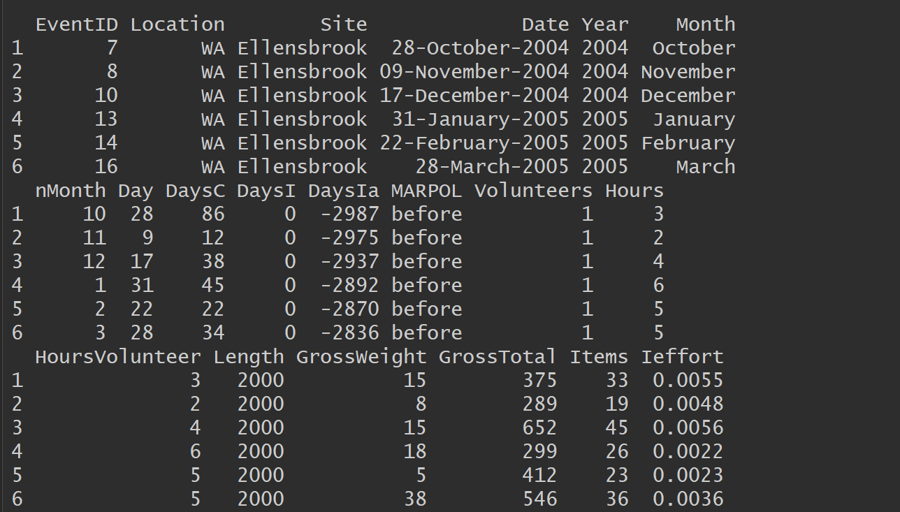
Here’s the head of the data:

Description of each one of the varables in the dataframe:

eventid = each sampling (clean-up) event
Location = Queensland and New South Wales
Sites = all the 9 sampling beaches

Date = specific dates for the clean-up events (day-month-year)
Date1 = specific dates for the clean-up events (day-month-year) on the POSICXT format
Year= Year of sampling event (2004 to 2018)
Month= Month of the sampling event (jan to dec)
nMonth= a number was determined to the respective month of the sampling event (1 to 12)
Day= Day of sampling (1 to 31)
Days = Days since the first date of clean up = just another way of using the dates

MARPOL = before and after implementation (factor with 2 levels)
DaysC = days between sampling events for the same sites = number of days since the previous clean-up event
DaysI = Days since intervention, all the dates before implementation are zero, and after we count the number of days since the implementation date (1 jan 2013)
DaysIa= same as DayI but instead of zero for before the intervention we have negative values (days)

Items = number of fishing and shipping items counted in each clean-up event
Hours = hours spent by all volunteers together at each clean up event
Lenght = Lenght of beach sampled by all volunteers together at each clean up event
volunteers = all volunteers at each clean up event
HoursVolunteer = hours spent bt each volunteer at each clean up event (Hours/volunteers)
Ieffort = the items standarized by the effort (hours, volunteers and lenght)

GrossWeight = total weight of the all the items found (not just fishing and shipping debris)
GrossTotal = total amount of the all the items found (not just fishing and shipping debris)

---

Problems:

My data has a few problems:

1. I think I will need to fix the effects of seasonal variation (Monthly) and .
2. of possible spatial correlation (probability of finding an item is higher after finding one since they can come from the same ship).
3. How do I handle the fact that the measurements were not taken at a regular interval?

I was trying to use GAMs to analyse the data and see the trends over time. The model I came across is the following:

m4 <- gamm(Ieffort ~ s(DaysIa)+ MARPOL + s(nMonth, bs = "ps", k = 12), 
           random = list(Site = ~1, Location = ~1), data = d)

How can I handle the fact that the measurements were not taken at a regular interval, the seasonality and the possible spatial correlation? Am I on the right track?

Answer 1

I would suggest a different strategy, fitting this as a GAM via gam(), and using a count distribution as the real response variable is an integer count.

The response should be Items in this setting. We do need to standardise by the effort but we can do that using a offset in the model. An offset is a term that has a fixed coefficient of 1, and it's inclusion in the model ends up standardising the response per unit effort, without having to do the standardisation yourself ahead of time. You will need to create an effort variable first though:

d <- transform(d, effort = Hours * Volunteers * Length)

Now we can use a count response model, such as the Poisson or a Negative Binomial, or even more exotic models like zero-inflated or hurdle count models. We must include the offset variable in the model on the scale of the link function. For most count models this will on the log scale by default, but do check implementations. You add an offset by adding

+ offset(log(effort))

to the model formula.

For the seasonal term, is there a reason for choosing a p-spline? I would normally use a cyclic spline, often a cyclic cubic spline bs = 'cc' but mgcv also offers a cyclic p-spline in more recent versions bs = 'cp'. You should also set knots for this term to avoid December and January from having the same estimated value. The idea here is that 1 and 12 will represent the mid-points of Jan and Dec respectively. Hence we want the spline to actually join at 0.5 and 12.5. To do this create a list, say knots with a named element for the nMonth variable and set the knot endpoints:

knots <- list(nmonth = c(0.5, 12.5))

We will use this when fitting the model.

m <- gam(Items ~ MARPOL + s(Site, bs = 're') + s(DaysIa, k = 20) + 
           s(nMonth, bs = 'cc', k = 12) + offset(log(effort)),
         data = d, family = poisson(link = 'log') + knots = knots)

This is a starting model (assuming that the change over time is encoded in DaysIa variable), with terms for,

• MARPOL before/after
• random effect for Site (I'm ignoring any nesting for Site within Location, but that could be done),
• smooth of change over time,
• smooth for seasonal effect, assumed constant here over the 15 year period,
• offset to standardise the Items response for effort.

You could extend this, for example to allow for separate random smooths per Site for DaysIa and nMonth if needed

m <- gam(Items ~ MARPOL + s(Site, bs = 're') + 
           s(DaysIa, Site, bs = 'fs', k = 20) + 
           s(nMonth, Site, bs = 'fs', xt = list(bs = 'cc'), k = 12) + 
           offset(log(effort)),
         data = d, family = poisson(link = 'log') + knots = knots)

If you want the seasonal effect to change with time, you might want nMonth and Year to interact smoothly, or just interact (convert Year to be a factor fYear and have a random nMonth smooth per level of fYear).

To explore this more, you may need to explain in a little more detail what you are trying to do specifically.

The spatial component here is not really modelled as a spatial term at all; what we're doing is saying that some locations / sites have a higher rate of Items than others. If there is a spatial component to this then you'd want something in the model to say that locations / sites closer to one another will have similar rates of Items. You may need to explain what we can use to model the Site effect spatially as it isn't clear to me how you want to account for this.

This model doesn't account for unmodelled temporal correlation; how we'd do that isn't clear to me just yet as we have several time variables in the model or available to us.

The model doesn't really care about the irregularity (but you would need to handle that when modelling residual temporal autocorrelation) in sampling.

I can also imagine that there is some information in knowing how many items were collected previously; say a ship has shed it's load and on day 4 the first few items come ashore, with increasing numbers of items washing up for the next say 10 days before tailing off again. You might want to consider if you want to include lagged-terms into the model, or just interpret a wiggly trend in DaysIa as accounting for this effect. In which case, you might need to increase k considerably — check that with gam.check().