Bayesian inference about means, observing only the sum of two random variables

Question

I have: $X \sim \mathcal{N}(\mu_x, \sigma_x^2)$ and $Y \sim \mathcal{N}(\mu_y, \sigma_y^2)$. $X$ and $Y$ are independent.
$\mu_x$ and $\mu_y$ are not known and I want to learn about them (Bayesian inference).
However, I don't observe draws from $X$ and $Y$ independently, I only observes draws of $Z = X + Y$, with $Z \sim \mathcal{N}(\mu_x + \mu_y, \sigma_x^2 + \sigma_y^2)$.

Given some prior about $\mu_x$ and $\mu_y$ (e.g. $\mu_x \sim N(m^x_0, s^x_0)$ and $\mu_y \sim N(m^y_0, s^y_0)$), can I get a posterior that would have a closed form (and which would also be normal - i.e. keep the conjugacy property) ?

I tried to do the computations, basically I'm stuck. If you know $\mu_x$ or $\mu_y$ it's quite straightforward because then you just change $Z$ into $Z - \mu_x$ for example.
But with both unknown I cannot get a normal closed form for the posterior (of $\mu_x$ or $\mu_y$) because the posterior depends on the other mean (which is also unknown).
e.g. for $\mu_x$ for example, the posterior is $\mu_x \sim N(m^x_1, s^x_1)$ where:
$s^x_1 = (1/\sigma^2_x + 1/s_x^2)^{-1}$
$m^x_1 = s^x_1 \Big( m^x_0/s_x^2 + (z - \mu_y)/\sigma^2_x \Big)$
But obviously, $\mu_y$ is not known either, hence the problem. The posterior must be weighted by your belief about $\mu_y$ somehow. And I'm not sure how it works. (Because similarly, your belief about $\mu_y$ is updated exactly in the same way). As suggested in the comments, there might be some identification problem here. But I'm not sure because the prior's precision limits the scope of your posterior about both distributions.

My questions are:
- Am I missing a simplification in the computations? i.e. maybe there is an additional simplification at the end.
- If no, is there another distribution that I could use (e.g. lognormal instead of normal? I thought maybe with the log properties I could factorize something) for which I would keep the conjugacy property?
- Does anyone have any source on this specific kind of learning setup?

EDIT: more details.

Answer 1

You are correct that $Z\mid \mu_x,\mu_y,\sigma^2_x,\sigma^2_y \sim \mathcal{N}(\mu_x + \mu_y, \sigma_x^2 + \sigma_y^2)$. First note that this likelihood is not identifiable. This is because $\mu_x,\mu_y$ will evaluate to the same function as $\mu_x-1,\mu_y+1$. Actually, you can add and subtract any number and get the same likelihood. This is why the likelihood has a “ridge.”

However, the posterior is identifiable. This means that any kind of inference about a single parameter will definitely be very sensitive to the prior you choose.

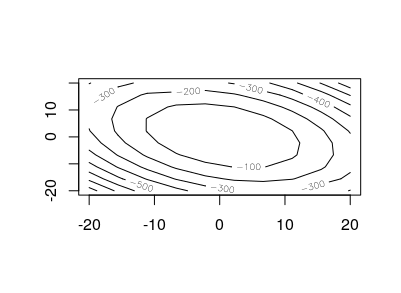
Assuming all of the variances are known, \begin{align*} p(z \mid \mu_x, \mu_y) &\propto p(z \mid \mu_x, \mu_y) p(\mu_x, \mu_y) \\ &\propto \exp\left[-\frac{(z- \mu_x - \mu_y)^2}{2\sigma^2_x + 2 \sigma^2_y} \right] \exp\left[-\frac{(\mu_x - m_0^x)^2}{2s_0^x} \right]\exp\left[-\frac{(\mu_y - m_0^y)^2}{2s_0^y} \right] \\ \end{align*} which is proportional to the exponential of $$ -\frac{1}{2(\sigma^2_x + \sigma^2_y)(s_0^x s_0^y)}\left\{ (z- \mu_x - \mu_y)^2s_0^xs_0^y + (\mu_x - m_0^x)^2s_0^y(\sigma^2_x + \sigma^2_y) + (\mu_y - m_0^y)^2s_0^x(\sigma^2_x + \sigma^2_y) \right\}. $$ This means that your posterior is bivariate normal, and after you collect the terms with $\mu_x\mu_y$, you'll see you'll get a negative correlation. This makes intuitive sense, because if $\mu_x$ is really "big", then that will probably mean $\mu_y$ is really "small."

Here's some R code that helps show this. It plots the log of the unnormalized posterior

# library(devtools)
# devtools::install_github("tbrown122387/mmcmc")
library(mmcmc)
logUnNormPosterior <- function(mux,muy){
  z <- 2
  sigmaSqX <- sigmaSqY <- sx <- sy <- 1
  mx <- my <- 0
  dnorm(x = z, mux+muy, sqrt(sigmaSqY + sigmaSqY), log = T)+
    dnorm(mux, mx, sx, log = T) + dnorm(muy, my, sy, log = T)
}
mmcmc::plotSurface(lowerFirst = -20, upperFirst = 20, 
                   lowerSecond = -20, upperSecond = 20,
                   numGridPointsOnEachAxis = 10, 
                   f = logUnNormPosterior, contour = T)

Here's the plot: