Calibration of correlation

Question

Let's say there are two random variables (for example, two time series data of S&P500 and a stock) and their correlation is 0.95. What is the best way to reduce the correlation between these two variables to 0.7, while keeping one as it is? One approach that comes to mind is to add noise (error terms). But how would I know what should the mean standard deviation for the noise? I would appreciate if one could show how to do this in R.

Answer 1

So if $\rho_N$ is the desired Pearson correlation, $\rho_0$ is the current correlation with $\rho_N\le \rho_0$, and $\epsilon$ is our uncorrelated noise:

$\frac{cov(X+\epsilon,Y)}{\sqrt{var(X+\epsilon)\sigma^2_Y}}=\rho_N$

Solving for variance of $\epsilon$

$\sigma^2_\epsilon=\frac{cov(X,Y)^2}{\rho_n^2\sigma_Y^2}-\sigma^2_X=\sigma_X^2\bigg(\frac{\rho_0^2}{\rho_N^2}-1\bigg)$

So, for your example, you'd be setting the variance of the noise to be $\approx .357\sigma_X^2$.

(may want to double check my algebra here)

Answer 2

Given the intended application, you might be interested in creating realistic modifications of the series of data.

Overview

This is easier to do than you might think. (See the three-line function decorrelate in the code below.) The idea is to generate the "noise" series realistically, according to any model you like. (You can even use actual data, such as a series for another stock or a portion of the series for the same stock at a different time.) The desired amount of correlation reduction determines what multiple of the noise series you need to add in order to achieve the intended reduction in correlation.

Analysis

To be explicit, let's suppose you have paired series $(x_t,y_t)$ and can produce a third series $\epsilon_t$ to use for the noise. Let the correlation coefficient of $(x_t,y_t)$ be $\rho$ and suppose you wish to obtain a new series $(y^*_t)$ (with the same average value as $(y_t)$) whose correlation with $(x_t)$ is $\kappa\rho.$ I assume $|\kappa|\lt 1:$ that is, you intend to reduce the correlation.

As a technical preliminary, intended to ensure you will be able to obtain an answer, we need first to "decorrelate" the noise from the original series. This is readily done with ordinary least squares regression: fit the model $E[\epsilon] = \beta_0 + \beta_x x + \beta_y y$ to the data and replace the series $(\epsilon_t)$ with the residuals of that model, found by subtracting its fitted values from the original values. Let $(e_t)$ be the residual series. (If you're truly unlucky, this series could be entirely zero: that would mean the "noise" was originally a linear combination of $(x_t)$ and $(y_t).$ In such a case you will have to come up with a different noise series and try again.) As a bonus, including the constant term $\beta_0$ in the model guarantees the average value of $(e_t)$ is zero, so that adding the noise does not change the overall level of the data.

The new series will be obtained by adding some positive multiple $\lambda$ of the noise to either $(y_t)$ (when $\kappa \ge 0$) or to $(-y_t)$ (when $\kappa \lt 0,$ which means you want to reverse the direction of correlation). That is, the solution will be

$$(y_t^*) = (\operatorname{sgn}(\kappa) y_t + \lambda e_t).$$

The value of $\lambda$ is found by comparing the correlation coefficients. The requirement (when $\kappa \gt 0$) is

$$\operatorname{Cor}(x_t, y_t^*) = \frac{\operatorname{Cov}(x_t, y_t + \lambda e_t)}{\sqrt{\operatorname{Var}(x_t) \operatorname{Var}(y_t+\lambda e_t)}} = \kappa \rho .$$

Writing $\sigma^2$ for the variance of $(x_t),$ $\tau^2$ for the variance of $(y_t),$ and $\psi^2$ for the variance of $(e_t),$ this equation becomes

$$\frac{\rho\sigma\tau}{\sigma \sqrt{\tau^2+\lambda^2\psi^2}} = \kappa \rho.$$

If $\rho=0$ there's nothing to do, and when $\rho\ne 0$ this conveniently simplifies (when squared) to

$$\frac{1}{1+\lambda^2\psi^2/\tau^2} = \kappa^2,$$

with the unique solution

$$\lambda = \frac{\tau}{\psi}\sqrt{\frac{1}{\kappa^2}-1}.$$

It's easy to verify this works for negative $\kappa$ as well.

To implement this in R, I offer the decorrelate function at the beginning of the code below. At line 2, it performs the decorrelation step using lm and residuals. It invisibly divides by $\psi$ using the scale function (also on line 2), but otherwise directly reflects the foregoing formula (line 3). For convenience, if you have no definite noise series $(\epsilon_t)$ to supply, it will create one randomly (out of Normal white noise, line 1).

---

Examples

First, here is the solution using the default white noise.

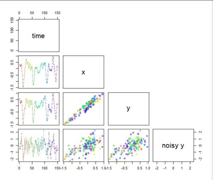
In this scatterplot matrix, the original series $(x_t)$ is at the top upper left plotted against time. It exhibits noticeable positive serial correlation: it's not jagged and random, but smoothly undulating. Beneath it are $(y_t)$ (also serially correlated) and then--this is the first solution, down in the lower left corner--the noisy version of $(y_t).$ (The rest of the matrix displays correlations among the series as scatterplots. The colors consistently show the times.)

The original correlation of $\rho=0.95$ has been reduced to precisely $\kappa \rho = 0.60.$ However, there's a problem: qualitatively, the noisy series doesn't look much like $(y_t).$ It's too jagged.

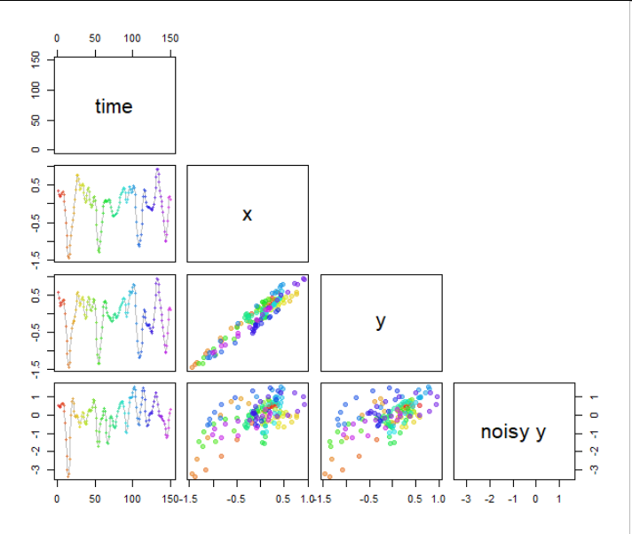
We solve this by using a noise series that has (approximately) the same serial correlation as $(y_t).$ Here's what the second solution looks like:

Look at the lower left corner. Once again, the correlation of this modified series $(y_t^*)$ with $(x_t)$ is precisely $\kappa \rho=0.60.$ If that seems like an improvement, then this method is probably what you want to use.

---

Code

Here is the R code that generated the data and the figures. You can modify its parameters to experiment. When you have real data, you only need the code starting at "Reduce their correlation" (as well as the decorrelate function, of course).

The mysterious part (in the middle) is the generation of a series $(x_t,y_t)$ with specified correlation. This is carried out by applying the algorithm to the series $(x_t,x_t),$ for which the correlation is $1,$ and reducing that correlation by an amount $\rho.$ I am pleased with this trick :-).

# Multiply the absolute correlation between `x` and `y` by a factor `kappa`
# by adding noise to `y`.  Returns the noisy `y`.
#
decorrelate <- function(x, y, kappa, noise) {
  if (missing(noise)) noise <- rnorm(length(x))
  eps <- c(scale(residuals(lm(noise ~ x + y))))
  y * sign(kappa) + eps * sd(y) * sqrt(1/kappa^2 - 1)
}
#
# Create MA time series data.  A Gaussian window of length 2w+1 is run over an iid 
# standard normal series to create a sequence of `n` values.
#
ts.create <- function(n, w) convolve(rnorm(n+2*w), dnorm((-w):w, 0, 2), type="filter")
#
# Create correlated data.
# set.seed(17)
rho <- 0.95
n <- 150
w <- 19
x <- convolve(rnorm(n+2*w), dnorm((-w):w, 0, 2), type="filter")
y <- decorrelate(x, x, rho, noise=ts.create(n, w))
#
# Reduce their correlation.
#
rho.new <- 0.60
y.star <- decorrelate(x, y, rho.new / rho, noise=ts.create(n, w))
#
# Graph the series and show their scatterplots.
#
f <- function(x, y) {
  if (diff(range(x))+1==length(x)) {cex=0.7; lines(x,y,col="Gray")} else cex=1
  points(x,y, pch=19, cex=cex, col=hsv(seq(0, 5/6, length.out=length(x)), .9, .9, .5))
}
pairs(cbind(time=seq_along(x), x, y, `noisy y`=y.star), upper.panel=NULL, lower.panel=f)

Answer 3

First, since OP's problem is with relation to stock and index returns correlation, I must note that one thing to be aware of is that if the stock, such as AAPL, is a part of index such as SPX, then the problem is a little more complex, because any change to AAPL will spill into SPX index.

So, let's assume that the stock in question is not a constituent of SPX index. In this case I offer you two and half methods. First two would preserve the index as is, and the last one will not, but it will not add external noise either.

mix-in noises with one variable staying the same

I can transform one of the variables in such a way that the other stays the same but correlation changes. It's a simple mixing in the noise from first variable into the second. This is how you do it.

Get new series Y as from original series X by solving for a and b: $$y_1=x_1\\ y_2=ax_1+bx_2\\var[y_2]=var[x_2]=\sigma_2^2\\cov[x_1,x_2]=\rho\sigma_1\sigma_2\\cov[y_1,y_2]=c\sigma_1\sigma_2$$

Write down variance and covariance of $y_2$: $$var[y_2]=a^2\sigma_1^2+b^2\sigma_2^2+2ab\rho\sigma_1\sigma_2\equiv\sigma_2^2$$ $$cov[y_1,y_2]=a\sigma_1^2+b\rho\sigma_1\sigma_2=c\sigma_1\sigma_2$$ $$a\sigma_1+b\rho\sigma_2=c\sigma_2$$

You have two nonlinear equations and two unknowns a,b. You can solve this analytically or like me, a lazy guy, numerically with Excel solver, which got me:

• a = 1.375
• b = -2.0213

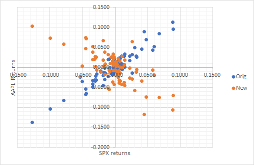
and the following plot of new series, where you can see that SPX returns remained the same and only AAPL returns changed while mean and variance were preserved:

Here's the first four moments after the transformation:

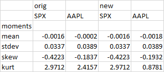
Note, that only kurtosis has changed significantly, yet it's a very important moment in portfolio management, for it is responsible for a lot of tail risk. In this case, the tail of the second variable thinnedconsiderably.

re-ordering variables

Second method is to not change the observations at all, but instead rearrange the observations in variables in such a way that correlation changes. Consider this: if I take random samples from both series, and calculate the correlation between these samples, then correlation will be zero. So, simple rearranging the order in variables will change correlation.

Advantage of this method is that variances remain the same, and overall distributions remain intact in the dataset. Since, you work with stock return, there's no autocorrelation, so rearranging doesn't impact this aspect at all, at least in theory. I don't know whether this method can generate drastic changes in correlation such flipping its sign like in the example above.

shuffling noise around

Instead of adding noise, let's push it around! We'll shuffle noise between two variables so that the correlation is what we want while preserving variances of each variable. Here's the final result for S&P 500 and Apple returns in 2020 Jan-Apr, where original correlation was 94% which I changed into -70%:

I used PCA and Cholesky decomposition to do this:

• apply PCA to destandardized original series X to get the uncorrelated series F
• standardize PC factors F to get unit variance series U
• apply Cholesky decomposition to standardized uncorrelated series U to obtain correlated series Y with unit variance
• destandardize Y to get to the series with original means and variances X'

This looks a bit intimidating, but you don't have to do this manually, and can use software. We don't introduce external noise. We only push the noise that exists in the data already from one place to another. Total variance of the data set remains the same as well as some other characteristics such as means.

Here's the first 4 moments after the transformation:

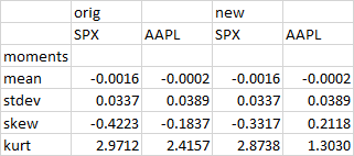
You can see how the higher moments change, especially, kurtosis. If the stock returns were normal, then this wouldn't have happened. However, the stock return usually have heavier tails than normal. So, watch out for thinner tails if you are analyzing tail risk metrics.