Time-to-ruin in the discrete-time random walk: From your question, I take it that you are referring to a discrete-time version of the gambler's ruin problem. Without loss of generality we can consider the wealth of the gambler denominated in units equivalent to the betting amount. We will assume that the wealth of the gambler is a positive whole number of such units, and we denote the starting wealth as $w_0 \in \mathbb{N}$. Then the time-to-ruin is defined as:
$$T \equiv \min \{ t \in \mathbb{N} | w_t = 0 \},$$
where the wealth follows the unit random walk process:
$$w_t = w_0 + \sum_{i=1}^t \Delta_i
\quad \quad \quad \mathbb{P}(\Delta_i = -1) = \mathbb{P}(\Delta_i = 1) = \frac{1}{2}.$$
The time-to-ruin is the "hitting time" for the state $w=0$ in this stochastic process. You can determine the distribution of the time-to-ruin by looking at the distributions of the hitting times. Here it is useful to appeal to a special result for random walks called the "hitting time theorem" (see e.g., Van Der Hofstad and Keane 2008 and Kager 2017), which shows that:
$$\mathbb{P}(T=t) = \frac{w_0}{t} \cdot \mathbb{P}(w_t = 0).$$
Below we will use this result to derive a useful distribution that is closely related to the distribution of the time-to-ruin. The result is a discrete phase-type distribution, which is a type of distribution used to model the hitting time to the absorbing state of a Markov chain.
Deriving the distribution of the time-to-ruin: Looking at the nature of the random walk, it is easy to see that the time-to-ruin must occur somewhere over the support $t = w_0, w_0 + 2, w_0 + 4, w_0 + 6, ...$. This is quite an intuitive result --- we need to have at least $w_0$ bets to lose the starting wealth, and any additional bets leading to ruin must come in pairs, each with one win and one loss cancelling each other out. Thus, to facilitate our analysis, it is useful to work with the total number of winning bets in the time-to-ruin:
$$R \equiv \frac{T - w_0}{2},$$
which has support $r = 0,1,2,3,...$. Now, applying the hitting time theorem above, we get:
$$\begin{align}
\mathbb{P}(R=r)
= \mathbb{P} \Bigg( \frac{T - w_0}{2} = r \Bigg)
&= \mathbb{P} ( T = w_0 + 2r ) \\[6pt]
&= \frac{w_0}{w_0 + 2r} \cdot \mathbb{P} ( w_{w_0 + 2r} = 0 ) \\[6pt]
&= \frac{w_0}{w_0 + 2r} \cdot \mathbb{P} \Bigg( w_0 + \sum_{i=1}^{w_0 + 2r} \Delta_i = 0 \Bigg) \\[6pt]
&= \frac{w_0}{w_0 + 2r} \cdot \mathbb{P} \Bigg( \sum_{i=1}^{w_0 + 2r} \mathbb{I}(\Delta_i=1) = r \Bigg) \\[6pt]
&= \frac{w_0}{w_0 + 2r} \cdot \text{Bin} ( r | w_0 + 2r, \tfrac{1}{2} ) \\[6pt]
&= \frac{w_0}{w_0 + 2r} \cdot \frac{(w_0 + 2r)!}{(w_0+r)! r!} \cdot \frac{1}{2^{w_0 + 2r}} \\[6pt]
&= \frac{w_0}{2^{w_0}} \cdot \frac{(w_0 + 2r - 1)!}{(w_0+r)! r!} \cdot \frac{1}{4^r} \\[6pt]
\end{align}$$
It is simplest to frame the gambler's ruin problem in terms of this distribution. However, we can convert back to the distribution for $T$. For any value $t = w_0, w_0 + 2, w_0 + 4, w_0 + 6, ...$ in the support for the time-to-ruin, we have:
$$\mathbb{P}(T=t) = w_0 \cdot \frac{(t - 1)!}{(\tfrac{t+w_0}{2})! (\tfrac{t-w_0}{2})!} \cdot \frac{1}{2^t}.$$
Implementation in R: We can program this density function using standard syntax for probability distribution as follows. In this function the input t is a vectorised input for the time-to-ruin. The function produces density values by default, but you can use the log input to produce log-densities instead.
druintime <- function(t, w, log = FALSE) {

  #Check inputs
  if (!is.numeric(t))           { stop('Error: Input t should be numeric') }
  if (!is.numeric(w))           { stop('Error: Input w must be a positive integer') }
  if (length(wealth) != 1)      { stop('Error: Input w must be a single value') }
  if (as.integer(w) != w)       { stop('Error: Input w must be a positive integer') }
  if (min(wealth) < 1)          { stop('Error: Input w must be a positive integer') }
  if (!is.logical(log))         { stop('Error: Input log must be a logical value') }
  if (length(log) != 1)         { stop('Error: Input log must be a single value') }

  #Compute number of successes in each time-to-ruin
  #and set indicators for integer values
  n   <- length(t)
  r   <- (t - w)/2
  IND <- (as.integer(r) == r)&(r >= 0)

  #Compute log-density
  LOGDEN <- rep(-Inf, n)
  LOGDEN[IND] <- log(w) - log(w + 2*r[IND]) +
                 dbinom(r[IND], size = w + 2*r[IND], prob = 1/2, log = TRUE)

  #Give output
  if (log) { LOGDEN } else { exp(LOGDEN) } }
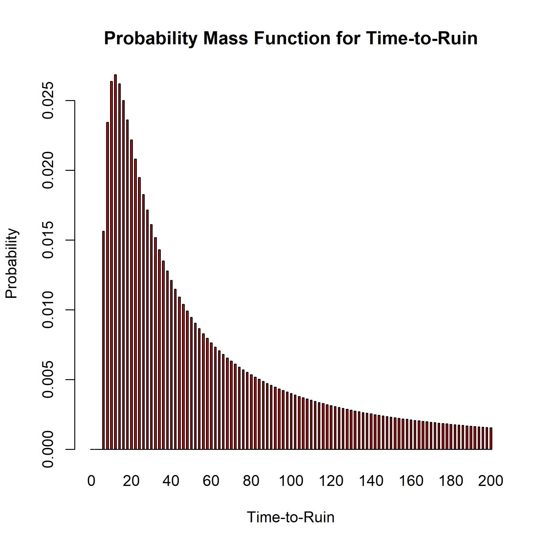
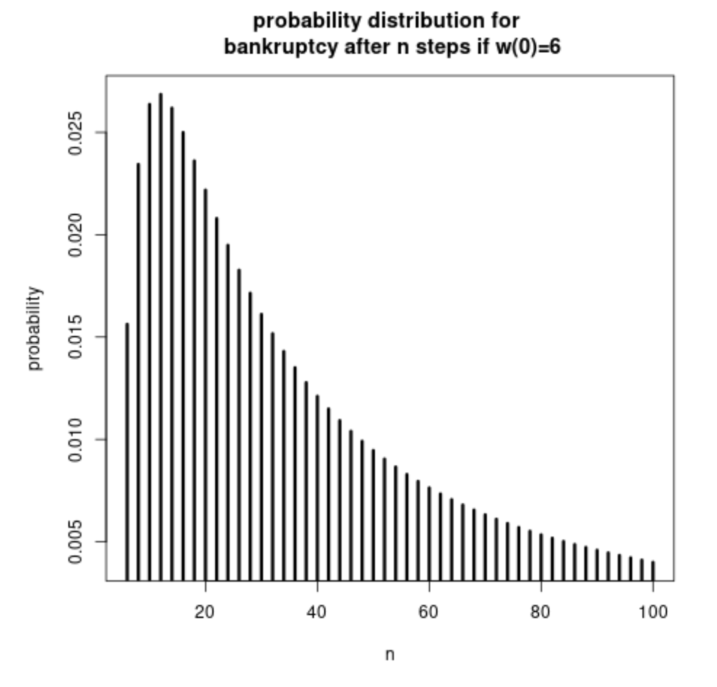
Implementing this with starting wealth $w_0 = 6$ gives the following probability mass function.
#Compute probability mass function over a set of input values
t    <- 0:200
w0   <- 6
DENS <- druintime(t, w = w0)

#Plot the mass function
t.names <- rep(NA, length(t))
for (i in 0:20) { t.names[1+10*i] <- t[1+10*i] }
barplot(DENS, names.arg = t.names,
        main = 'Probability Mass Function for Time-to-Ruin', col = 'red',
        xlab = 'Time-to-Ruin', ylab = 'Probability')


