18
$\begingroup$

Gaussian data distributed in a single dimension requires two parameters to characterise it (mean, variance), and rumour has it that around 30 randomly-selected samples is usually sufficient to estimate these parameters with reasonably high confidence. But what happens as the number of dimensions increases?

In two dimensions (e.g. height, weight) it takes 5 parameters to specifiy a "best-fit" ellipse. In three dimensions, this rises to 9 parameters to describe an ellipsoid, and in 4-D it takes 14 parameters. I am interested to know if the number of samples required to estimate these parameters also rises at a comparable rate, at a slower rate or (please no!) at a higher rate. Better still, if there was a broadly accepted rule of thumb that suggests how many samples are required to characterise a gaussian distribution in a given number of dimensions, that would be good to know.

To be more precise, suppose we want to define a symmetrical "best-fit" boundary centred at the mean point inside which we can be confident that 95% of all samples will fall. I want to know how many samples it might take to find the parameters to approximate this boundary (interval in 1-D, ellipse in 2-D, etc) with suitably high (>95%) confidence, and how that number varies as the number of dimensions increases.

$\endgroup$
11
  • 3
    $\begingroup$ Without a sufficiently precise definition of 'pin down', it's not really possible to answer this question even for a univariate Gaussian. $\endgroup$
    – Glen_b
    Commented May 19, 2013 at 22:37
  • 1
    $\begingroup$ How about: how many samples does it take to be at least 95% confident that 95% of all samples (but only 95% of all samples) will lie within a defined interval/ellipse/ellipsoid/hyperellipsoid? $\endgroup$
    – omatai
    Commented May 19, 2013 at 23:11
  • 1
    $\begingroup$ That is to say... 95% of all samples will lie within some defined distance of the mean. How many samples are required to define that distance (interval/ellipse/ellipsoid/etc) with 95% or better confidence? $\endgroup$
    – omatai
    Commented May 19, 2013 at 23:17
  • 1
    $\begingroup$ Ah, you now have a relatively standard type of question; you should probably edit your original question to reflect your intent more clearly. $\endgroup$
    – Glen_b
    Commented May 19, 2013 at 23:22
  • 2
    $\begingroup$ As soon as you have one more independent data value than there are parameters (whence $\binom{d+2}{2}$ values in $d$ dimensions), you can erect a 95% confidence region around them. (One can do even better using non-traditional techniques.) That's an answer--it's a definitive one--but it's probably not what you're looking for. The point is that you need to stipulate some absolute scale of desired accuracy in order to obtain an answer to this question. $\endgroup$
    – whuber
    Commented May 30, 2013 at 23:00

3 Answers 3

13
$\begingroup$

The amount of data needed to estimate the parameters of a multivariate Normal distribution to within specified accuracy to a given confidence does not vary with the dimension, all other things being the same. Therefore you may apply any rule of thumb for two dimensions to higher dimensional problems without any change at all.

Why should it? There are only three kinds of parameters: means, variances, and covariances. The error of the estimate in a mean depends only on the variance ($\sigma^2$) and the amount of data ($n$). Thus, when $(X_1, X_2, \ldots, X_d)$ has a multivariate Normal distribution and the $X_i$ have variances $\sigma_i^2$, then the estimates of $\mathbb{E[X_i]}$ depend only on the $\sigma_i$ and $n$. Whence, to achieve adequate accuracy in estimating all the $\mathbb{E}[X_i]$, we only need to consider the amount of data needed for the $X_i$ having the largest of the $\sigma_i$. Therefore, when we contemplate a succession of estimation problems for increasing dimensions $d$, all we need to consider is how much the largest $\sigma_i$ will increase. When these parameters are bounded above, we conclude that the amount of data needed does not depend on dimension.

Similar considerations apply to estimating the variances $\sigma_i^2$ and covariances $\sigma_{ij}$: if a certain amount of data suffice for estimating one covariance (or correlation coefficient) to a desired accuracy, then--provided the underlying normal distribution has similar parameter values--the same amount of data will suffice for estimating any covariance or correlation coefficient.


To illustrate, and provide empirical support for this argument, let's study some simulations. The following creates parameters for a multinormal distribution of specified dimensions, draws many independent, identically distributed sets of vectors from that distribution, estimates the parameters from each such sample, and summarizes the results of those parameter estimates in terms of (1) their averages--to demonstrate they are unbiased (and the code is working correctly--and (2) their standard deviations, which quantify the accuracy of the estimates. (Do not confuse these standard deviations, which quantify the amount of variation among estimates obtained over multiple iterations of the simulation, with the standard deviations used to define the underlying multinormal distribution!) My claim is that these standard deviations do not materially change when the dimension $d$ changes, provided that as $d$ changes, we do not introduce larger variances into the underlying multinormal distribution itself.

The sizes of the variances of the underlying distribution are controlled in this simulation by making the largest eigenvalue of the covariance matrix equal to $1$. This keeps the probability density "cloud" within bounds as the dimension increases, no matter what the shape of this cloud might be. Simulations of other models of behavior of the system as the dimension increases can be created simply by changing how the eigenvalues are generated; one example (using a Gamma distribution) is shown commented out in the R code below.

What we are looking for is to verify that the standard deviations of the parameter estimates do not appreciably change when the dimension $d$ is changed. I therefore show the results for two extremes, $d=2$ and $d=60$, using the same amount of data ($30$) in both cases. It is noteworthy that the number of parameters estimated when $d=60$, equal to $1890$, far exceeds the number of vectors ($30$) and exceeds even the individual numbers ($30*60=1800$) in the entire dataset.

Let's begin with two dimensions, $d=2$. There are five parameters: two variances (with standard deviations of $0.097$ and $0.182$ in this simulation), a covariance (SD = $0.126$), and two means (SD = $0.11$ and $0.15$). With different simulations (obtainable by changing the starting value of the random seed) these will vary a bit, but they will consistently be of comparable size when the sample size is $n=30$. For instance, in the next simulation the SDs are $0.014$, $0.263$, $0.043$, $0.04$, and $0.18$, respectively: they all changed but are of comparable orders of magnitude.

(These statements can be supported theoretically but the point here is to provide a purely empirical demonstration.)

Now we move to $d=60$, keeping the sample size at $n=30$. Specifically, this means each sample consists of $30$ vectors, each having $60$ components. Rather than list all $1890$ standard deviations, let's just look at pictures of them using histograms to depict their ranges.
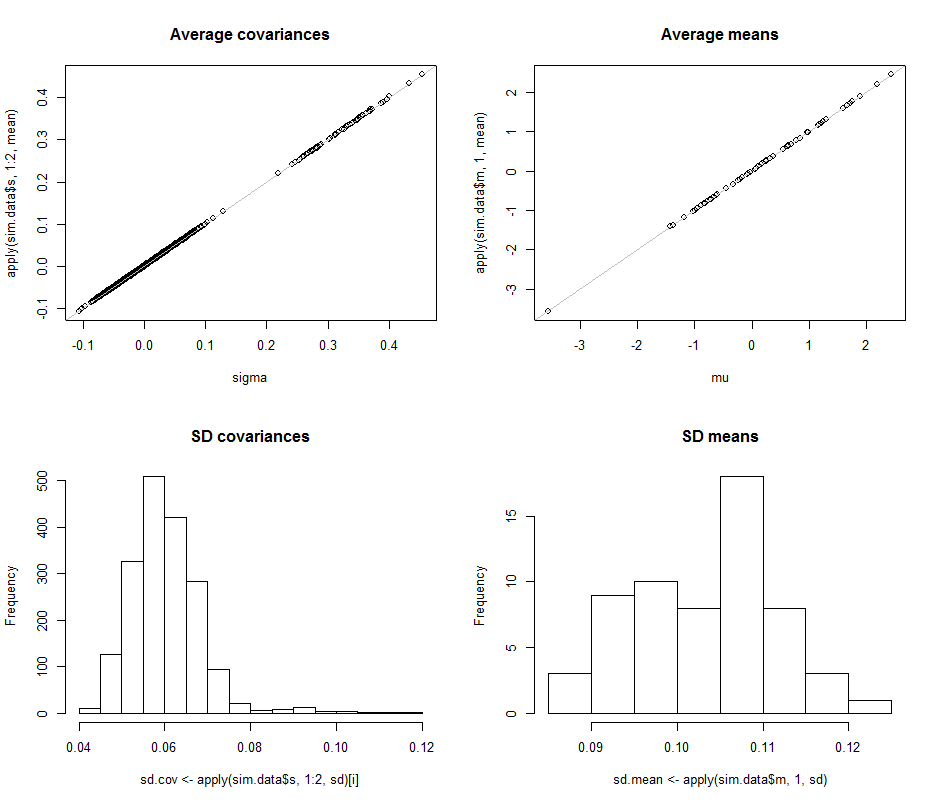
Figure

The scatterplots in the top row compare the actual parameters sigma ($\sigma$) and mu ($\mu$) to the average estimates made during the $10^4$ iterations in this simulation. The gray reference lines mark the locus of perfect equality: clearly the estimates are working as intended and are unbiased.

The histograms appear in the bottom row, separately for all entries in the covariance matrix (left) and for the means (right). The SDs of the individual variances tend to lie between $0.08$ and $0.12$ while the SDs of the covariances between separate components tend to lie between $0.04$ and $0.08$: exactly in the range achieved when $d=2$. Similarly, the SDs of the mean estimates tend to lie between $0.08$ and $0.13$, which is comparable to what was seen when $d=2$. Certainly there's no indication that the SDs have increased as $d$ went up from $2$ to $60$.

The code follows.

#
# Create iid multivariate data and do it `n.iter` times.
#
sim <- function(n.data, mu, sigma, n.iter=1) {
  #
  # Returns arrays of parmeter estimates (distinguished by the last index).
  #
  library(MASS) #mvrnorm()
  x <- mvrnorm(n.iter * n.data, mu, sigma)
  s <- array(sapply(1:n.iter, function(i) cov(x[(n.data*(i-1)+1):(n.data*i),])), 
        dim=c(n.dim, n.dim, n.iter))
  m <-array(sapply(1:n.iter, function(i) colMeans(x[(n.data*(i-1)+1):(n.data*i),])), 
            dim=c(n.dim, n.iter))
  return(list(m=m, s=s))
}
#
# Control the study.
#
set.seed(17)
n.dim <- 60
n.data <- 30    # Amount of data per iteration
n.iter <- 10^4  # Number of iterations
#n.parms <- choose(n.dim+2, 2) - 1
#
# Create a random mean vector.
#
mu <- rnorm(n.dim)
#
# Create a random covariance matrix.
#
#eigenvalues <- rgamma(n.dim, 1)
eigenvalues <- exp(-seq(from=0, to=3, length.out=n.dim)) # For comparability
u <- svd(matrix(rnorm(n.dim^2), n.dim))$u
sigma <- u %*% diag(eigenvalues) %*% t(u)
#
# Perform the simulation.
# (Timing is about 5 seconds for n.dim=60, n.data=30, and n.iter=10000.)
#
system.time(sim.data <- sim(n.data, mu, sigma, n.iter))
#
# Optional: plot the simulation results.
#
if (n.dim <= 6) {
  par(mfcol=c(n.dim, n.dim+1))
  tmp <- apply(sim.data$s, 1:2, hist)
  tmp <- apply(sim.data$m, 1, hist)
}
#
# Compare the mean simulation results to the parameters.
#
par(mfrow=c(2,2))
plot(sigma, apply(sim.data$s, 1:2, mean), main="Average covariances")
abline(c(0,1), col="Gray")
plot(mu, apply(sim.data$m, 1, mean), main="Average means")
abline(c(0,1), col="Gray")
#
# Quantify the variability.
#
i <- lower.tri(matrix(1, n.dim, n.dim), diag=TRUE)
hist(sd.cov <- apply(sim.data$s, 1:2, sd)[i], main="SD covariances")
hist(sd.mean <- apply(sim.data$m, 1, sd), main="SD means")
#
# Display the simulation standard deviations for inspection.
#
sd.cov
sd.mean
$\endgroup$
2
  • 1
    $\begingroup$ so.....how many samples do I need? Related question is here -- math.stackexchange.com/questions/4169322/… $\endgroup$ Commented Jun 10, 2021 at 18:34
  • $\begingroup$ @YaroslavBulatov Please see our posts on power analysis. I'm confident the answer has appeared many times for the question of estimating means. For estimating variances and covariances, you might not be able to find an answer--and that's worth asking in a separate thread. Likewise, more complex situations (such as a sample size needed to estimate a linear combination of mean and variance) would need to be discussed separately. $\endgroup$
    – whuber
    Commented Jan 8, 2022 at 17:44
1
$\begingroup$

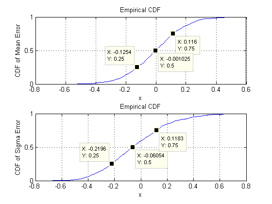
Some brief numerics gives the following error distributions for the fit of 30 samples created from a standard normal distribution then fit to a univariate Gaussian.

enter image description here

The quartiles are indicated. It is assumed that this level of variation is desired in the multi-dimensional case.

I don't have the time to beat up MatLab to get the total result, so I will share my "rule of thumb". The 30 is provided as a rule of thumb, or heuristic so it is assumed that heuristics are not unacceptable.

My heuristic is to use Pascal's triangle multiplied by the univariate case. enter image description here

If I am using 2d data then I go to the 2nd row and sum it to get 2x the number of samples, or 60 samples. For 3d data I go to the 3rd row and sum it to get 4x the number of samples or 120 samples. For 5d data I go to the 5th row and sum it to get 16x the number of samples, or 480 samples.

Best of luck.

EDIT:

It was intuitive, but everything has to be defended in math. I can't just take leaps from formulation of polynomial forms from Finite Elements with experience to get a ballpark.

The equation for the sum of the $ k^{th}$ row of Pascal's triangle is $ 2^k$.

My idea for the approach here is to equate the AIC of a higher-dimensional distribution with more samples to a reduced dimensional distribution with fewer samples.

The Akaike Information Criterion (AIC) is defined as $ AIC = n \log( \frac {RSS}{n}) + 2*k$ where $ RSS$ is residual sum of squares, $ n$ is sample count, and $ k$ is parameter count for the model.

$ AIC_1 = AIC_2$

$ n_1 \log(\frac {RSS_1}{n_1}) +2k_1 = n_2 \log(\frac {RSS_2}{n_2}) +2k_2$

For each dimension that we eliminate this means that the mean loses a row and the covariance loses both a row and a column. We can state this as

$ k \left( d\right)= d^2+d$.

of

$k \left( d+1 \right) - k \left( d\right) = 2 d + 2$

Assuming the error per sample point is constant relates the residual sum of squares to the sample count, and the term in the logarithm stays constant. The difference in sample count becomes a scaling constant.

so we have:

$ n_1 A +2(k_2+2d+2) = n_2 A +2k_2 $

solving for the increase in samples with dimension gives:

$ n_2- n_1 = (2(k_2+2d+2) - 2k_2) A^{-1} = (4 d+4 ) \cdot A^{-1} $

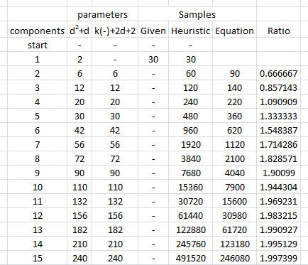
So what is the scaling function? Lets assume that for a 2-dimensional multivariate Gaussian the number of samples required is 15 per parameter. There are 2 means and 4 elements of the covariance therefore 6 parameters or 90 samples. The difference is 60 samples, the value of $ A^{-1} = 5$.

enter image description here

At this point I would say that the heuristic starts a little low but ends up being about 2x the number of samples required. Its range of best utility, in my personal opinion, is around 4 dimensions or so.

EDIT:

So I have read the answer of @whuber and I like it. It is empirical, and in this case that is authoritative. I voted for his answer.

In the following I am attempting to discuss and hoping to be able to use more than ~300 characters, and I am hoping to be able to embed pictures. I am therefore discussing within the bounds of the answer. I hope this is okay.

I am at this point not convinced that use of AIC for this, or how sample size and parameter sizes were used was incorrect.

Next steps:

  • replicate @whuber's results, confirm them empirically
  • Test the AIC, at least in some ensemble sense, to confirm whether it is appropriate
  • If AIC is appropriate, then try to use empirical methods to chase down flaw in reasoning.

Comments and suggestions welcome.

$\endgroup$
13
  • 4
    $\begingroup$ Could you provide some justification for your heuristic? $\endgroup$
    – whuber
    Commented Jun 3, 2013 at 19:09
  • 1
    $\begingroup$ And could you confirm that the sum of the 5th row is in fact 16? $\endgroup$
    – omatai
    Commented Jun 3, 2013 at 22:50
  • $\begingroup$ 1+4+6+4+1 = 1 + 10 + 5 = 16. Sorry about that. 16 $ \ne$ 22. I must have been half-asleep when I added. $\endgroup$ Commented Jun 3, 2013 at 22:54
  • 1
    $\begingroup$ How do you come up with $2^{d+1}-2$ for the number of parameters? That's far too many. For instance, with $d=9$ components only $54$ parameters are needed (for $9$ means, $9$ covariances, and $36$ correlations). This could explain why your recommendation calls for such an extraordinarily high sample size! $\endgroup$
    – whuber
    Commented Jun 4, 2013 at 18:14
  • 1
    $\begingroup$ @whuber, I find that I learn more by my errors (after I learn of them) than by my being correct. Surprisingly enough, being wrong feels exactly like being right until I know that I am wrong. Thank you. ted.com/talks/kathryn_schulz_on_being_wrong.html $\endgroup$ Commented Jun 7, 2013 at 16:50
0
$\begingroup$

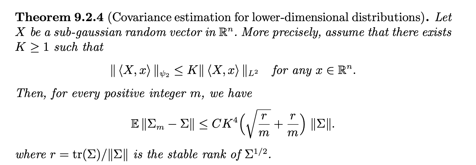
Theorem 9.2.4 from Vershynin's "High Dimensional Probability" book gives a dimension-free sample complexity of estimating covariance matrix

$\endgroup$

Your Answer

By clicking “Post Your Answer”, you agree to our terms of service and acknowledge you have read our privacy policy.

Not the answer you're looking for? Browse other questions tagged or ask your own question.