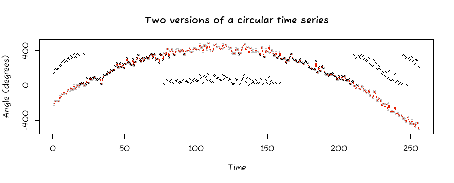
One way (out of many) is to adjust the data by whole periods to make them vary more continuously over time.
Specifically, modify the time series $(x)=(x_1,x_2,\ldots,)$ to a time series $(y)=(y_1,y_2,\ldots)$ that is congruent to $(x)$ modulo the period $\tau.$ Begin with $$y_1=x_1 + k\tau$$ where $k$ is any integer you choose to make $y_1$ a "nice" starting value. At each successive time $i+1,$ predict $y_{i+1}$ as $\hat y_{i+1} = y_i$ and then adjust it modulo $\tau$ to make the prediction as close as possible to the observed value:
$$y_{i+1} = x_{i+1} + \left[\frac{\hat y_{i+1} - x_{i+1}}{\tau}\right]\tau.\tag{*}$$
The bracket $[\ ]$ means to round to the nearest integer.
It is explicit in these two formulas that for every $i,$ $y_i$ differs from $x_i$ by an integral multiple of $\tau.$ Thus, $(y)$ is a valid representative of $(x).$ This construction makes successive values of $y_i$ as close as possible to what you might expect based on the preceding values: that's what I mean by "more continuously."
This is simple to code. In R for example, with the time series data in a vector x, create the adjusted vector y with
tau <- 360                             # ... or 2*pi or whatever
y <- x                                 # Allocates storage for `y`
k <- -1; y[1] <- x[1] %% tau + k * tau # Optional: `k` should be integral
for (i in seq_along(y)[-1]) y[i] <- x[i] + tau * round((y[i-1] - x[i]) / tau)
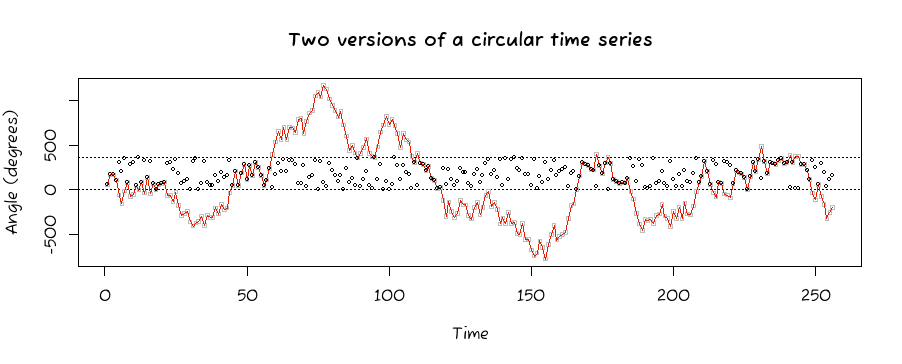
Now you may simply plot $(y).$ If you like, overplot the original data $(x).$ In this figure $(x)$ is plotted as black circles and $(y)$ as gray squares, connected by red line segments.

The results might be meaningless with highly noisy data but they can still be helpful:

If there is some kind of underlying continuity, you now have a chance of seeing it while still displaying the original data.
Of course, if you have a model for the time series that lets you forecast one step into the future, you might do better by forecasting $y_{i+1}$ from preceding values rather than using the naive forecast embodied in $(*).$ If you don't have a model, you might consider modeling $(y)$ rather than $(x)$ and then (if $(y)$ is very noisy) iterating the modification procedure $(*)$ using this provisional model. The idea is that $(y)$ is likely a better manifestation of the evolution of the data over time than is $(x)$ and studying it might reveal information lost by recording $(x)$ modulo $\tau.$ This opens up the entire world of time series modeling techniques to analyze circular data, at very little cost.


