1
$\begingroup$

I have a longitudinal study with two time points (before/after), whereas a particular score was standardized across all individuals and time points, and thus provided only in terms of z-scores. (Edit: to clarify, "before"-data and "after"-data were pooled before the standardization, not a separate standardization for "before"-data and another for "after"-date).

I read this paper regarding longitudinal standardization ("Don't"), but still - I want to try and see whether the score was (statistically significantly) positively or negatively changed when comparing the "before" and "after" groups.

For example, suppose we have the following subset of a table:

ID Z-Score Before Z-Score After
1000 +2 +0.1
1001 -1 +1
1002 -0.5 +0.2

My understanding is that z-scores cannot be subtracted and then averaged. Therefore, my thoughts were:

  • Taking all "before" and "after" datapoints, and applying a Mann-Whitney on the two groups. This ignores the "matching" of the data.
  • Converting all z-score to percentiles, then calculating difference and applying a t-test on the difference:
ID Percentile Before Percentile After Percentile Diff
1000 0.977249868 0.539827837 -0.437422031
1001 0.158655254 0.841344746 0.682689492
1002 0.308537539 0.579259709 0.270722171

Am I correct in my assumptions? Is this a valid method? Are there any better methods? (Assume that I cannot reproduce the data that was used to calculate the z-score).

$\endgroup$

1 Answer 1

1
$\begingroup$

Perhaps you are trying to unbury some data that doesn't exist in raw form. In any case, I don't think its a good idea to standardize the data and then run mean/rank difference tests.

Doing any form of t-test here wouldn't work on standardized data for the simple reason that the mean will by definition equal zero for both groups, and so it follows there will be no statistically significant difference. Converting the z-scores to percentiles doesn't fix this issue because you are now just testing location differences in the same way. A ranked test doesn't fix this issue either for the reasons you stated already. As proof of that, here are those tests on simulated data in R.

#### Sim Data ####
library(tidyverse)
set.seed(123)
x <- rnorm(100,mean=50,sd=10)
y <- rnorm(100,mean=60,sd=10)
df <- data.frame(x,y)

data <- df %>% 
  gather() %>% 
  as_tibble()
data

#### Test ####
t.test(data$value ~ data$key,
       paired=T)

#### Standardize ####
zx <- scale(x)
zy <- scale(y)
zdf <- data.frame(zx,zy)

zdata <- zdf %>% 
  gather() %>% 
  as_tibble()
zdata

#### Test Again ####
t.test(zdata$value ~ zdata$key,
       paired=T)

#### Percentiles ####
px <- pnorm(zx)
py <- pnorm(zy)
pdf <- data.frame(px,py)
pdata <- pdf %>% 
  gather() %>% 
  as_tibble()
pdata

#### Test Once More ####
t.test(pdata$value ~ pdata$key,
       paired=T)

The first t-test on raw data shows what we expect, a statistically significant difference:

    Paired t-test

data:  data$value by data$key
t = -5.8876, df = 99, p-value = 5.379e-08
alternative hypothesis: true mean difference is not equal to 0
95 percent confidence interval:
 -10.723482  -5.317464
sample estimates:
mean difference 
      -8.020473 

The second test of z-scores is fairly nonsensical, as now the mean difference is zero (or very very close to it with floating points shown by the scientific notation), and thus $p = 1$:

    Paired t-test

data:  zdata$value by zdata$key
t = 7.6905e-16, df = 99, p-value = 1
alternative hypothesis: true mean difference is not equal to 0
95 percent confidence interval:
 -0.2874763  0.2874763
sample estimates:
mean difference 
   1.114216e-16

Percentile differences have similar issues:

    Paired t-test

data:  pdata$value by pdata$key
t = 0.2507, df = 99, p-value = 0.8026
alternative hypothesis: true mean difference is not equal to 0
95 percent confidence interval:
 -0.07050474  0.09089738
sample estimates:
mean difference 
     0.01019632 

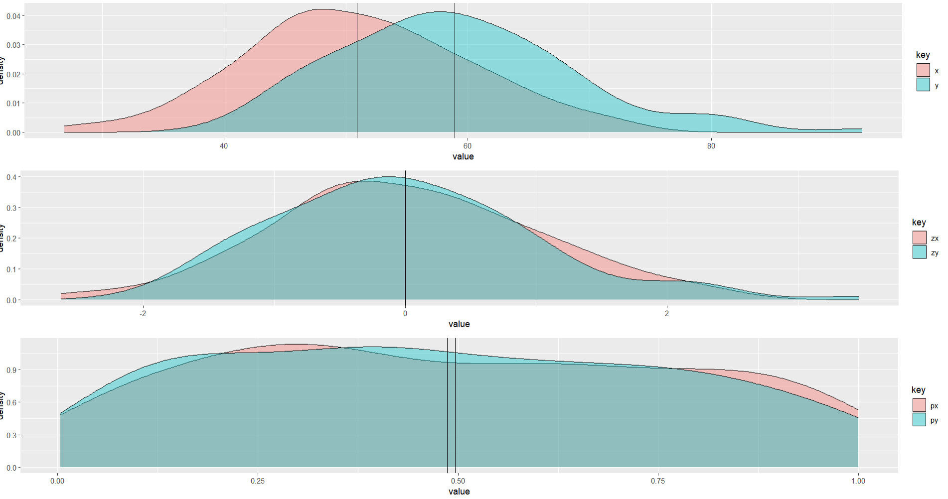
If you mean that you want to run a t-test on the difference scores of percentiles alone, this isn't possible because you are only using one vector of scores (there is no comparison to another group). To get a sense of what this looks like visually, here is the code to plot their densities:

#### Plot Them ####
p1 <- data %>% 
  ggplot(aes(x=value,
             fill=key))+
  geom_density(alpha=.4)+
  geom_vline(xintercept = mean(x))+
  geom_vline(xintercept = mean(y))

p2 <- zdata %>% 
  ggplot(aes(x=value,
             fill=key))+
  geom_density(alpha=.4)+
  geom_vline(xintercept = mean(zx))+
  geom_vline(xintercept = mean(zy))

p3 <- pdata %>% 
  ggplot(aes(x=value,
             fill=key))+
  geom_density(alpha=.4)+
  geom_vline(xintercept = mean(px))+
  geom_vline(xintercept = mean(py))

ggpubr::ggarrange(p1,p2,p3,ncol = 1)

Whereas the first plot shows the actual mean differences (the black line running down the middle), the other two have nonsensical mean differences now:
enter image description here

$\endgroup$
6
  • $\begingroup$ Sorry, I believe I was misunderstood. I meant the standardization process was performed for the entire dataset, "before" and "after" together, not separately for the "before" and the "after" groups. I'll clarify that in the main post as well. $\endgroup$ Commented Nov 27, 2023 at 22:46
  • $\begingroup$ I'm even more confused now. The entirety of the raw scores were transformed into a single distribution of z-scores? That makes even less sense than simply z-score transforming them separately. $\endgroup$ Commented Nov 28, 2023 at 0:38
  • $\begingroup$ Indeed, all raw scores were transformed into a single distribution. Actually, the dataset is larger, as there are more before&after scores (Let's call them Before2, After2, Before3, After3) which are not necessary for the question at hand - I only need to compare "Before1" and "After1". I think this was done to mitigate the differences between "before" and "after" and to compare the three different scores (which I don't need for my study, but believe this was the rationale behind the pooled standardization). $\endgroup$ Commented Nov 28, 2023 at 14:18
  • $\begingroup$ The problem is that they are treating the distributions as the same. Which they're not. If you can't find the raw data, idk what utility this data will have for your purposes. $\endgroup$ Commented Nov 28, 2023 at 22:33
  • $\begingroup$ OK. To wrap it up - as I understand from you, if the normalization was done after pooling both "Before" and "After" together, there is no way to determine whether "Before" is statistically significantly higher or lower than "After"? $\endgroup$ Commented Nov 30, 2023 at 19:08

Your Answer

By clicking “Post Your Answer”, you agree to our terms of service and acknowledge you have read our privacy policy.

Not the answer you're looking for? Browse other questions tagged or ask your own question.