Should the within-subject variability decrease?

Question

I have a crossover experiment design, detailed as follows.

1. there are 7 sites conducting the same experiment;
2. In the experiment of each sites, 5 different treatments are administered to $n_i, \, (i = 1, 2, \dots, 7)$ subjects during 5 different periods. The $n_i$'s are not necessarily equal;
3. In this experiment, only the fixed treatment effect and random subject effect are of interest. Other effects are ignored.

The variance of the random subject effect is thus the between-subject variability, and the remaining variability from experiment error is within-subject variability.

Three mixed-effects models in terms of different sites are investigated.

(1) Site 1 and 2 combined; (2) Sites other than 1 and 2; (3) All sites.

In each mixed-effect model, fixed treatment effect and random subject effect are specified. After running the three models, I got to know that the within-subject variability for the three are,

(1) 0.7904; (2) 0.8203; (3) 0.8526

respectively.

However, I was told that there results should NOT be like this. Instead, intuitively the within-subject variability from Model (3) should be less than that from Model (2). The argument is that since Model (1) has the smallest within-subject variability, then if we combine the sites (subjects) in Model (1) with those in Model (2), which results to Model (3), we should expect the within-subject variability decrease.

I am not convinced by this the simple intuition. My questions are:

(1) Is the above argument against the results correct?

(2) Are there clearer intuitions that help explain this problem?

(3) Are there any proofs or arguments from theoretical aspect (I mean by derivations) to help understand this?

EDIT:

My description to the problem might not be quite clear. But you can think of subjects from site 1 and 2 are of high quality control since the Model (1) produces lower within-subject variability. Thus the rational which is against the current numerical results is, if these "better" subjects are combined with others (Site 3 to 7), it's expected the within-subject variability decrease. Thus the within-subject variability from Model (3) should be smaller than that of Model (2). What I am asking is whether this rational necessarily holds. If so, how? If not, then why?

END EDIT

---

EDIT-2:

I am posting some "made-up" data for anyone who might be curious about. It's of longitudinal type. There are four variables "Subject", "Treatment", "Site", and response variable "y". As I said above, each site has some subjects for the experiment. There are 5 different treatment levels, denoted as A, B, C, D, and E.

The model is pretty simple, as shown in following sample SAS code, with fixed treatment effect and random subject effect. Intentionally, I am not considering other effects (like site effect). The code applies to all three models, except that the "data = case2" corresponds to different (sub)sets of data with different sites included.

proc mixed data = case2 asycov cl covtest plots;
class Subject   Treatment;
model y= Treatment/solution;
random Subject;
lsmeans TRT/pdiff cl;
run;

Here is the sample data.

Subject Treatment   Site    y
1-1     D              1    5.68387
1-1     E              1    5.65
1-1     C              1    4.45098
1-1     A              1    0.79048
1-1     B              1    4.50455
1-2     C              1    4.13208
1-2     D              1    5.10459
1-2     B              1    4.34468
1-2     E              1    5.07556
1-2     A              1    2.36296
1-3     B              1    -0.77037
1-3     C              1    0.59167
1-3     A              1    -1.53191
1-3     D              1    3.42
1-3     E              1    2.89231
...
2-1     D              2    4.80312
2-1     E              2    5.60606
2-1     C              2    5.38
2-1     A              2    0.39474
2-1     B              2    3.97714
2-2     C              2    4.46667
2-2     D              2    5.73333
2-2     B              2    6.17391
2-2     E              2    4.86957
2-2     A              2    -0.02
...
...
7-1     E              7    4.4875
7-1     A              7    -2.10667
7-1     D              7    5.71579
7-1     B              7    1.17895
7-1     C              7    0.97576
7-2     D              7    3.05083
7-2     E              7    3.25473
7-2     C              7    2.7925
7-2     A              7    1.23
7-2     B              7    3.98769
7-3     C              7    4.32754
7-3     D              7    5.2875
7-3     B              7    4.46575
7-3     E              7    4.12787
7-3     A              7    0.61481

END EDIT-2

Any comments or ideas are welcome. Thanks in advance!

Answer 1

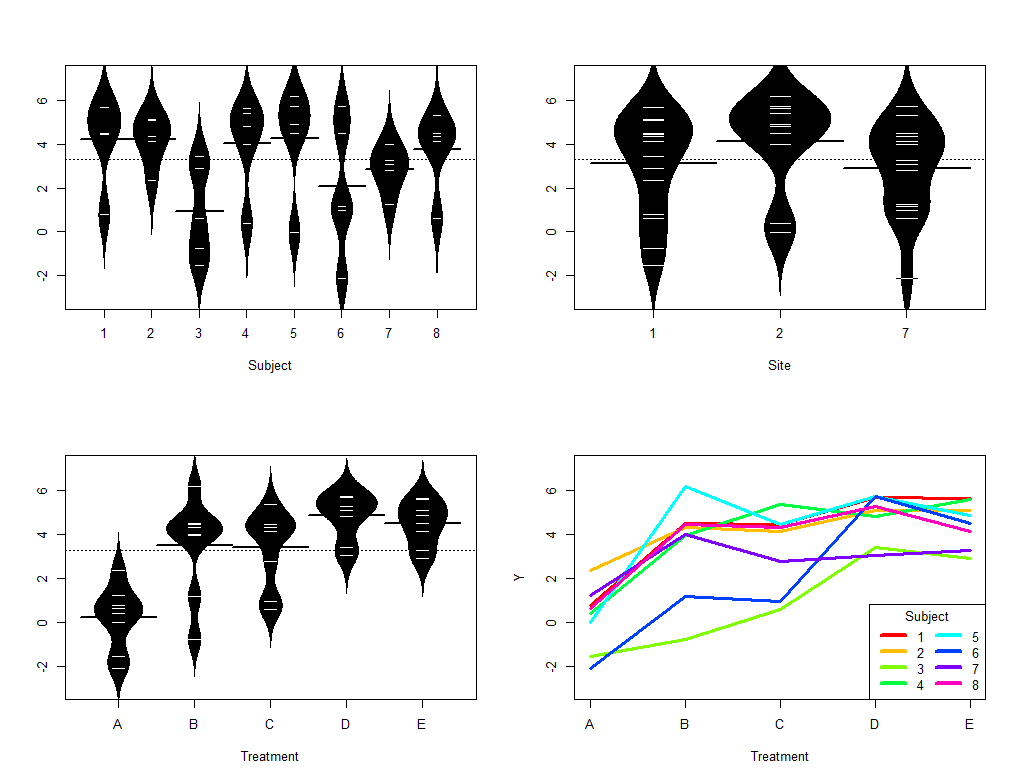
The situation is somewhat different from what I thought. In case someone else can answer it, here is the data and my understanding of (I do not know SAS well...) the analysis in R:

require(beanplot)
require(lme4)

dat.full<-structure(list(Subject = c(1L, 1L, 1L, 1L, 1L, 2L, 2L, 2L, 2L, 
2L, 3L, 3L, 3L, 3L, 3L, 4L, 4L, 4L, 4L, 4L, 5L, 5L, 5L, 5L, 5L, 
6L, 6L, 6L, 6L, 6L, 7L, 7L, 7L, 7L, 7L, 8L, 8L, 8L, 8L, 8L), 
    Treatment = structure(c(4L, 5L, 3L, 1L, 2L, 3L, 4L, 2L, 5L, 
    1L, 2L, 3L, 1L, 4L, 5L, 4L, 5L, 3L, 1L, 2L, 3L, 4L, 2L, 5L, 
    1L, 5L, 1L, 4L, 2L, 3L, 4L, 5L, 3L, 1L, 2L, 3L, 4L, 2L, 5L, 
    1L), .Label = c("A", "B", "C", "D", "E"), class = "factor"), 
    Site = c(1L, 1L, 1L, 1L, 1L, 1L, 1L, 1L, 1L, 1L, 1L, 1L, 
    1L, 1L, 1L, 2L, 2L, 2L, 2L, 2L, 2L, 2L, 2L, 2L, 2L, 7L, 7L, 
    7L, 7L, 7L, 7L, 7L, 7L, 7L, 7L, 7L, 7L, 7L, 7L, 7L), y = c(5.68387, 
    5.65, 4.45098, 0.79048, 4.50455, 4.13208, 5.10459, 4.34468, 
    5.07556, 2.36296, -0.77037, 0.59167, -1.53191, 3.42, 2.89231, 
    4.80312, 5.60606, 5.38, 0.39474, 3.97714, 4.46667, 5.73333, 
    6.17391, 4.86957, -0.02, 4.4875, -2.10667, 5.71579, 1.17895, 
    0.97576, 3.05083, 3.25473, 2.7925, 1.23, 3.98769, 4.32754, 
    5.2875, 4.46575, 4.12787, 0.61481)), .Names = c("Subject", 
"Treatment", "Site", "y"), class = "data.frame", row.names = c(NA, 
-40L))



par(mfrow=c(2,2))
beanplot(dat.full$y~dat.full$Subject, xlab="Subject", 
         ylim=c(min(dat.full$y)-1, max(dat.full$y)+1))
beanplot(dat.full$y~dat.full$Site, xlab="Site", 
         ylim=c(min(dat.full$y)-1, max(dat.full$y)+1))
beanplot(dat.full$y~dat.full$Treatment, xlab="Treatment", 
         ylim=c(min(dat.full$y)-1, max(dat.full$y)+1))

Nsubj<-length(unique(dat.full$Subject))
plot(0,0, type="n",xlim=c(1,5), xaxt="n", xlab="Treatment",
     ylab="Y",  ylim=c(min(dat.full$y)-1, max(dat.full$y)+1))
axis(side=1, at=as.numeric(unique(dat.full$Treatment)),
     labels=unique(dat.full$Treatment))
for(i in 1:Nsubj){
  sub<-dat.full[which(dat.full$Subject==unique(dat.full$Subject)[i]),]
  sub<-sub[sort(as.numeric(sub$Treatment), index.return=T)$ix,]
  lines(sub$Treatment,sub$y, col=rainbow(Nsubj)[i], lwd=3)
}
legend("bottomright", legend=unique(dat.full$Subject), col=rainbow(Nsubj), 
       lwd=4, title="Subject", ncol=2)


dat1<-dat.full[which(dat.full$Site %in% 1),]
dat27<-dat.full[which(dat.full$Site %in% c(2,7)),]

fit.all<-lmer(dat.full$y~dat.full$Treatment + (1|dat.full$Subject))
fit1<-lmer(dat1$y~dat1$Treatment + (1|dat1$Subject))
fit27<-lmer(dat27$y~dat27$Treatment + (1|dat27$Subject))

> fit.all
Linear mixed model fit by REML ['lmerMod']
Formula: dat.full$y ~ dat.full$Treatment + (1 | dat.full$Subject)
REML criterion at convergence: 127.467
Random effects:
 Groups           Name        Std.Dev.
 dat.full$Subject (Intercept) 1.142   
     Residual                     1.064   
Number of obs: 40, groups:  dat.full$Subject, 8
Fixed Effects:
        (Intercept)  dat.full$TreatmentB  dat.full$TreatmentC  
             0.2168               3.2660               3.1728  
dat.full$TreatmentD  dat.full$TreatmentE  
             4.6331               4.2786  
> fit1
Linear mixed model fit by REML ['lmerMod']
Formula: dat1$y ~ dat1$Treatment + (1 | dat1$Subject)
REML criterion at convergence: 37.0667
Random effects:
 Groups       Name        Std.Dev.
 dat1$Subject (Intercept) 1.8608  
 Residual                 0.8506  
Number of obs: 15, groups:  dat1$Subject, 3
Fixed Effects:
    (Intercept)  dat1$TreatmentB  dat1$TreatmentC  dat1$TreatmentD  
         0.5405           2.1524           2.5177           4.1956  
dat1$TreatmentE  
         3.9988  
> fit27
Linear mixed model fit by REML ['lmerMod']
Formula: dat27$y ~ dat27$Treatment + (1 | dat27$Subject)
REML criterion at convergence: 76.0409
Random effects:
 Groups        Name        Std.Dev.
 dat27$Subject (Intercept) 0.7462  
     Residual                  1.1876  
Number of obs: 25, groups:  dat27$Subject, 5
Fixed Effects:
     (Intercept)  dat27$TreatmentB  dat27$TreatmentC  dat27$TreatmentD  
         0.02258           3.93411           3.56592           4.89554  
dat27$TreatmentE  
         4.44657  

My understanding is that @AaronZeng wants to know under what conditions the residuals can be fit.all>fit27>fit1. This is not the case in the example data.