Generating random samples with bivariate t-copula

Question

I'm trying to generate a bivariate random sample of the t-copula (using rho = 0.8), without using the "copula" package and its function "rCopula" with method "tCopula". I'm using the following R-code:

N <- 10000
R <- array(c(1,0.8,0.8,1), dim=c(2,2))
L <- t(chol(R)) 
Z <- rbind(rnorm(N),rnorm(N)) 
X <- L%*%Z 
df <- 2
W <- df/rchisq(N,df)
Y <- sqrt(W)*X  
plot(Y[1,],Y[2,])
U <- pt(Y,df)
plot(U[1,],U[2,])

But the plot does not look like random points from a t-copula:

Does anyone know if I'm making a conceptual error or a mistake in the code?

It should look more like this: (generated using the copula package and its inbuilt functions)

Answer 1

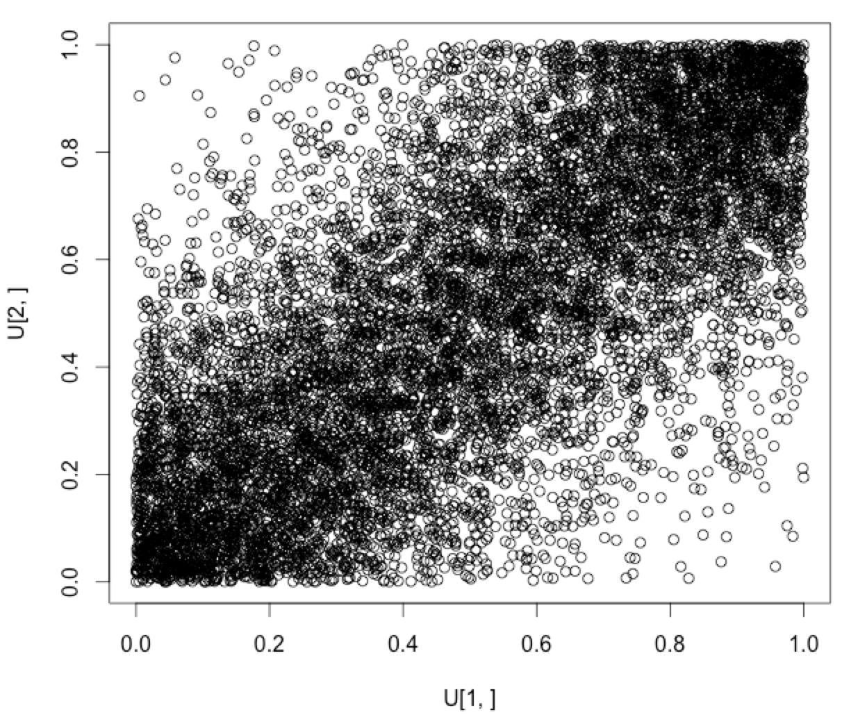
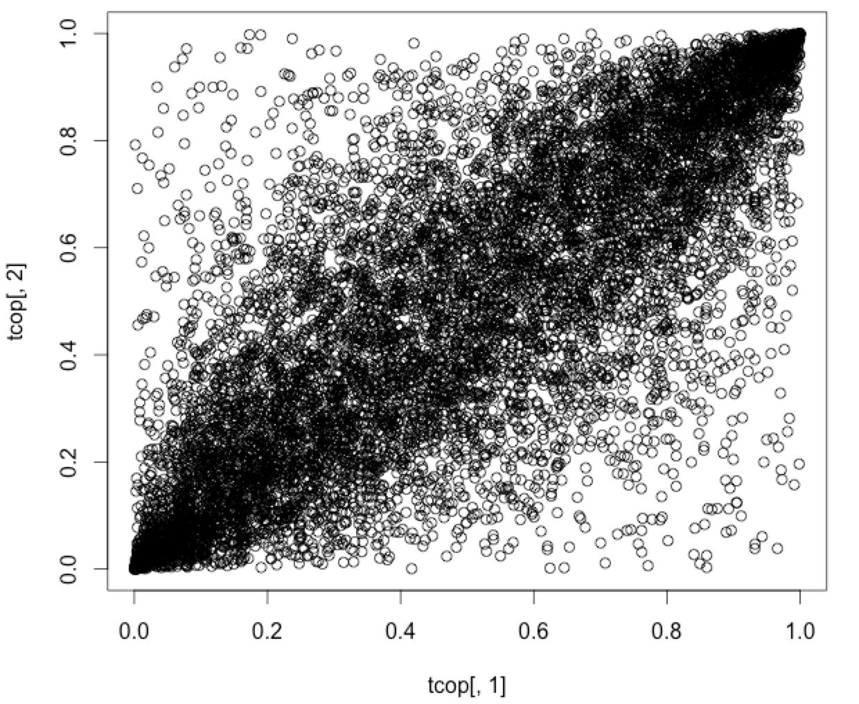
Despite their relative simplicity I've found it quite difficult to find a straightforward guide to copulas besides this short blog post. I went back through your code, fixed it up a bit and annotated what the steps were doing, but not why, as best I could if it should be of any use to others just starting out.

Update: After a bit more research I found this pdf, section 5 / pg 18 of which outlines pseudo code for a number of different copulas.

#a tcopula using rho = 0.8
#done from first principles
require(mvtnorm)
numObs <- 10000
#NX2 shaped matrix
initialObservations <- rmvnorm(numObs,mean=rep(0,2))

#this is a 2X2 symmetric matrix based off of rho=0.8 and is positive definite
psdRhoMatrix <- matrix(c(1,0.8,0.8,1),2,2)
#the transpose of the cholesky decomposition of the psdRhoMatrix
#which gives us a lower triangle matrix for some particular reason
lowerTriangleCholesky <- chol(psdRhoMatrix)

#this lower triangle matrix (for whatever reason) is able to make
#the observations in each column correlated
# NX2 = NX2 %*% 2X2
correlatedObservations <- initialObservations %*% lowerTriangleCholesky

degreesOfFreedom <- 2
#the meaning of this step eludes me, it's a vector of random chi-square observations.
#Maybe something to do with applying the inverse CDF.
randomChiSqrStep <- degreesOfFreedom/rchisq(numObs,degreesOfFreedom)
#transforming the correlated variables
#the random chiSquaredStep is applied to each column of the correlatedObservations
#for element wise multiplication to be properly applied the data needs to be
#sorted into columns rather than rows. NX2 = NX1 * NX2
penultimateTransformation <- sqrt(randomChiSqrStep) *  correlatedObservations
plot(penultimateTransformation[,1],penultimateTransformation[,2])

#run the fully transformed and correlated observations through the t-dist PDF and that's it
tCopulaOutPut <- pt(penultimateTransformation,degreesOfFreedom)
plot(tcopulaOutPut[,1],tcopulaOutPut[,2])

Answer 2

I found the mistake, it has to do with the element-wise multiplication in line 8. It should be

Y <- rbind(sqrt(W),sqrt(W))*X