How to interpret and do forecasting using tsoutliers package and auto.arima

Question

I have got monthly data from 1993 to 2015 and would like to do forecasting on these data. I used tsoutliers package to detect the outliers, but I do not know how do I continue to forecast with my set of data .

This is my code:

product.outlier<-tso(product,types=c("AO","LS","TC"))
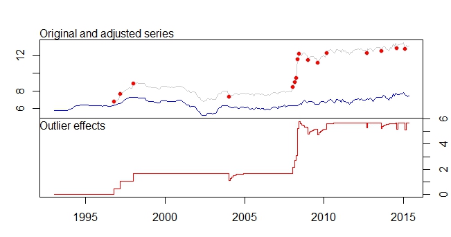
plot(product.outlier)

This is my output from tsoutliers package

ARIMA(0,1,0)(0,0,1)[12]                    

Coefficients:
        sma1    LS46    LS51    LS61    TC133   LS181   AO183   AO184   LS185   TC186    TC193    TC200
      0.1700  0.4316  0.6166  0.5793  -0.5127  0.5422  0.5138  0.9264  3.0762  0.5688  -0.4775  -0.4386
s.e.  0.0768  0.1109  0.1105  0.1106   0.1021  0.1120  0.1119  0.1567  0.1918  0.1037   0.1033   0.1040
       LS207    AO237    TC248    AO260    AO266
      0.4228  -0.3815  -0.4082  -0.4830  -0.5183
s.e.  0.1129   0.0782   0.1030   0.0801   0.0805

sigma^2 estimated as 0.01258:  log likelihood=205.91
AIC=-375.83   AICc=-373.08   BIC=-311.19

 Outliers:
    type ind    time coefhat  tstat
1    LS  46 1996:10  0.4316  3.891
2    LS  51 1997:03  0.6166  5.579
3    LS  61 1998:01  0.5793  5.236
4    TC 133 2004:01 -0.5127 -5.019
5    LS 181 2008:01  0.5422  4.841 
6    AO 183 2008:03  0.5138  4.592
7    AO 184 2008:04  0.9264  5.911
8    LS 185 2008:05  3.0762 16.038
9    TC 186 2008:06  0.5688  5.483
10   TC 193 2009:01 -0.4775 -4.624
11   TC 200 2009:08 -0.4386 -4.217
12   LS 207 2010:03  0.4228  3.746
13   AO 237 2012:09 -0.3815 -4.877
14   TC 248 2013:08 -0.4082 -3.965
15   AO 260 2014:08 -0.4830 -6.027
16   AO 266 2015:02 -0.5183 -6.442

I have these warning messages as well.

Warning messages:
1: In locate.outliers.iloop(resid = resid, pars = pars, cval = cval,  :
  stopped when ‘maxit’ was reached
2: In locate.outliers.iloop(resid = resid, pars = pars, cval = cval,  :
  stopped when ‘maxit’ was reached
3: In locate.outliers.oloop(y = y, fit = fit, types = types, cval = cval,  :
  stopped when ‘maxit’ was reached
4: In arima(x, order = c(1, d, 0), xreg = xreg) :
  possible convergence problem: optim gave code = 1
5: In auto.arima(x = c(5.77, 5.79, 5.79, 5.79, 5.79, 5.79, 5.78, 5.78,  :
  Unable to fit final model using maximum likelihood. AIC value approximated

Doubts:

1. If I am not wrong, tsoutliers package will remove the outliers it detect and through the use of the dataset with outliers removed, it will give us the best arima model suited for the data set, is it correct?
2. The adjust series data set is being shifted down by a lot due to remove of the level shift,etc. Doesn't this mean that if the forecasting is done on the adjusted series, the output of the forecast will be very inaccurate, since the more recent data are already more than 12, while adjusted data shift it to around 7-8.
3. What does warning message 4 and 5 means? Does it mean it cannot do auto.arima using the adjusted series?
4. What does the [12] in ARIMA(0,1,0)(0,0,1)[12] mean? Is it just my frequency/periodicity of my dataset, which I set it to monthly? And does this also means that my data series is seasonal as well?
5. How do I detect seasonality in my data set? As from the visualisation of the time series plot, I cant see any obvious trend, and if I use the decompose function, it will assume that there is a seasonal trend? So do I just believe what the tsoutliers tell me, where there is seasonal trend, since there is MA of order 1?
6. How do I continue to do my forecasting with this data after identifying these outliers?
7. How to incorporate these outliers to other forecasting models - Exponential Smoothing, ARIMA, Strutural Model, Random Walk, theta? I am sure I cannot remove the outliers since there are level shift, and if I only take adjusted series data, the values will be too small, so what do I do?

Do I need to add these outliers as regressor in the auto.arima for forecasting? How does this work then?

Answer 1

These comments are too long ...thus an "ANSWER"

1. You are wrong it does not adjust and then identify ARIMA (as AUTOBOX does).It presumtively assumes no intervention adjustment and then rushes to identify an ARIMA model potentially impacted by the non-treatment of anomalies. Often one needs to adjust for both user-specified causal series and/or unspecified deterministic structure (outliers/level shifts, seasonal pulses, local time trends) before identifying the ARIMA structure. See this example of a poor dignosis which makes the mistake of unnecessarily differencing the original series while the true/correct state of nature doesn't need any differencing. Non-stationarity does not necessarily imply the need for differencing but can often suggests de-meaning i.e.the adjustment for a change in level/mean

2. Correct forecasting is always done from the original series thus the forecast should be believable given the history.

3. I have no idea as I do not actively use this procedure. I recommended it to you because you asked for free r based solutions NOT because I thought it was good or sufficient as ARIMA modelling is an iterative (multi-stage) self-checking process.

4. the model suggests it thinks that the data has an ma(12) seasonal component BUT this could be simply reflect the need for a seasonal pulse.

5. the concept of a seasonal trend is at best vague .

6. My answer would be too obvious and self-effacing

Answer 2

The package 'tsoutliers' implements the procedure described in by Chen and Liu (1993) [1]. A description of the package and the procedure is also given in this document.

Briefly, the procedure consists of two main stages:

1. Detection of outliers upon a chosen ARIMA model.
2. Choose and/or refit the ARIMA model including the outliers detected in the previous step and remove those outliers that are not significant in the new fit.

The series is then adjusted for the detected outliers and the stages (1) and (2) are repeated until no more outliers are detected or until a maximum number of iterations is reached.

---

The first stage (detection of outliers) is also an iterative process. At the end of each iteration the residuals from the ARIMA model are adjusted for the outliers detected within this stage. The process is repeated until no more outliers are found or until a maximum number of iterations is reached (by default 4 iterations). The first three warnings that you get are related to this inner loop, i.e., the stage is exited after four iterations.

You can increase this maximum number of iterations through the argument maxit.iloop in function tso. It is advisable not to set a high number of iterations in the first stage and let the process move on to the second stage where the ARIMA model is refitted or chosen again.

---

The warnings 4 and 5 are related to the process of fitting the ARIMA model and chosen the model, respectively for functions stats::arima and forecast:auto.arima. The algorithm that maximizes the likelihood function does not always converge to a solution. You can find some details related to these issues, for example, in this post and this post

---

[1] Chung Chen and Lon-Mu Liu (1993) "Joint Estimation of Model Parameters and Outlier Effects in Time Series", Journal of the American Statistical Association, 88(421), pp. 284-297. DOI: 10.1080/01621459.1993.10594321.