Rank-deficiency means that we are unable to uniquely determine the relationship between response and covariates. The QR factorization with pivoting strategy used by lm ensures a unique solution in numerical point of view, but estimated coefficients do not match the truth, typically because it constrains some coefficients to 0. When using this set of coefficients for prediction, we can be away from truth.
In the following I will present a long simulation study with R.
In practice there could only be four scenarios:
- model matrix is full-rank, predictor matrix is full-rank;
- model matrix is full-rank, predictor matrix is rank-deficient;
- model matrix is rank-deficient, predictor matrix is full-rank;
- model matrix is rank-deficient, predictor matrix is rank-deficient.
In machine language terminology, the model matrix is the one associated with training dataset, and the predictor matrix is the one associated with test dataset. The following toy function generates two datasets (each with n data) for a regression model overall three numeric covariates and an intercept. model.rank1.defect and predictor.rank1.defect specify whether we want those matrices to be rank-1 deficient. The reason for using relatively few covariates are commented. The way to achieve deficiency is also commented. Note that the true model is generated on the complete dataset (of 2 * n data) which has full rank. A noise-to-signal ratio 0.1 is used.
sim <- function (n = 1000, model.rank1.defect = FALSE, predictor.rank1.defect = FALSE) {

  ## since we only impose rank-1 deficiency, we'd better try small number of parameters
  ## so that the degree of deficiency is relatively high
  ## We guess that higher degree of deficiency is,
  ## the easier we are going to spot "misleading" result in scatter plot
  p <- 3

  #############################
  ## similate a model matrix ##
  #############################

  ## generate a full rank model matrix
  Xm <- matrix(runif(n * p), n, p)
  ## make it rank-1 deficient if required
  if (model.rank1.defect) {
    # take a random column, replace it by the sum of remaining two columns
    ind <- sample(p, 1)
    Xm[, ind] <- rowSums(Xm[, -ind])
    }

  #################################
  ## similate a predictor matrix ##
  #################################

  ## generate a full rank predictor matrix
  Xp <- matrix(runif(n * p), n, p)
  ## make it rank-1 deficient if required
  if (predictor.rank1.defect) {
    # take a random column, replace it by the sum of remaining two columns
    ind <- sample(p, 1)
    Xp[, ind] <- rowSums(Xp[, -ind])
    }

  #########################
  ## assume a true model ##
  #########################

  beta <- rnorm(p)  ## true coefficients for covariates
  y.true <- 0.5 + rbind(Xm, Xp) %*% beta  ## intercept = 0.5
  y <- y.true + rnorm(2 * n, 0, sqrt(0.1 * var(y.true)))  ## noise to signal ratio = 0.1

  ###########################################
  ## separate training and testing dataset ##
  ###########################################

  train <- data.frame(y = y[1:n], X = I(Xm), y.true = y.true[1:n])
  test <- data.frame(y = y[-(1:n)], X = I(Xp), y.true = y.true[-(1:n)])

  ###########################################
  ## return datasets and true coefficients ##
  ###########################################

  list(train = train, test = test, coef = c(0.5, beta))
  }
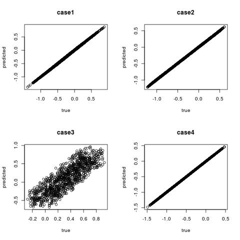
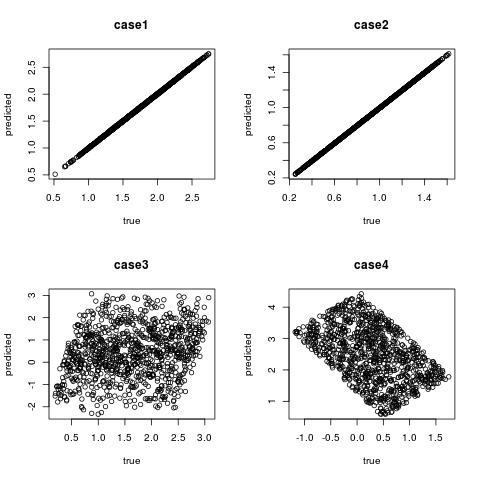
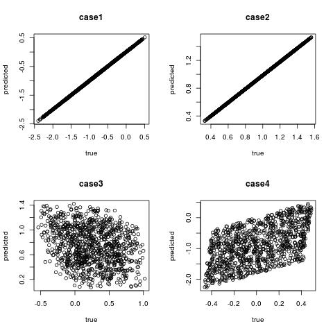
Basically we want to see how good / bad the prediction could be (compared with the truth) in four cases. The following function produces scattered plot for four cases, and note that good prediction means that the dots are scattered along y = x line.
inspect <- function (seed = 0, n = 1000) {

  set.seed(seed)

  case1 <- sim(n, model.rank1.defect = FALSE, predictor.rank1.defect = FALSE)
  case2 <- sim(n, model.rank1.defect = FALSE, predictor.rank1.defect = TRUE)
  case3 <- sim(n, model.rank1.defect = TRUE, predictor.rank1.defect = FALSE)
  case4 <- sim(n, model.rank1.defect = TRUE, predictor.rank1.defect = TRUE)

  par(mfrow = c(2, 2))

  fit1 <- lm(y ~ X, data = case1$train)
  plot(case1$test$y.true, predict(fit1, case1$test), main = "case1", xlab = "true", ylab = "predicted")

  fit2 <- lm(y ~ X, data = case2$train)
  plot(case2$test$y.true, predict(fit2, case2$test), main = "case2", xlab = "true", ylab = "predicted")

  fit3 <- lm(y ~ X, data = case3$train)
  plot(case3$test$y.true, predict(fit3, case3$test), main = "case3", xlab = "true", ylab = "predicted")

  fit4 <- lm(y ~ X, data = case4$train)
  plot(case4$test$y.true, predict(fit4, case4$test), main = "case4", xlab = "true", ylab = "predicted")

  list(case1 = rbind(truth = case1$coef, estimated = coef(fit1)),
       case2 = rbind(truth = case2$coef, estimated = coef(fit2)),
       case3 = rbind(truth = case3$coef, estimated = coef(fit3)),
       case4 = rbind(truth = case4$coef, estimated = coef(fit4)))
  }
It is generally a good idea to set a reasonably big n, say 1000, for clear visualization. You are recommended to try several random seeds, but I will just show the result for 0, 1, 2.
inspect(seed = 0, n = 1000)
#$case1
#          (Intercept)         X1        X2        X3
#truth       0.5000000 -0.5380638 0.4965946 -1.441966
#estimated   0.5086424 -0.5182216 0.4801427 -1.462437
#
#$case2
#          (Intercept)       X1        X2         X3
#truth        0.500000 1.683990 -1.544324 -0.1908871
#estimated    0.485759 1.690604 -1.529844 -0.1870299
#
#$case3
#          (Intercept)         X1         X2        X3
#truth       0.5000000 -0.8292477 0.04317512 0.4441213
#estimated   0.5144345 -1.2640980 0.47286008        NA
#
#$case4
#          (Intercept)         X1         X2        X3
#truth       0.5000000 -1.3502605 -0.2520004 0.9186201
#estimated   0.4857474 -0.4213176 -1.1679039        NA

inspect(seed = 1, n = 1000)
#$case1
#          (Intercept)        X1        X2       X3
#truth        0.500000 0.7391149 0.3866087 1.296397
#estimated    0.494829 0.7564111 0.3780248 1.302040
#
#$case2
#          (Intercept)        X1       X2         X3
#truth       0.5000000 0.1490125 1.572552 -0.4313906
#estimated   0.4926926 0.1454275 1.575065 -0.4292703
#
#$case3
#          (Intercept)        X1         X2       X3
#truth       0.5000000 0.2994154 -0.4803364 2.456836
#estimated   0.5033469 2.7558496 -2.9404693       NA
#
#$case4
#          (Intercept)        X1         X2        X3
#truth       0.5000000 0.5066593  0.7627762 -2.231709
#estimated   0.4883394 2.7323985 -1.4522909        NA

inspect(seed = 2, n = 1000)
#$case1
#          (Intercept)        X1         X2        X3
#truth       0.5000000 -2.138476 -0.9007918 0.1499151
#estimated   0.4996853 -2.147597 -0.8861852 0.1555451
#
#$case2
#          (Intercept)       X1         X2        X3
#truth       0.5000000 1.415801 -0.3443290 0.1640968
#estimated   0.4943133 1.424356 -0.3759823 0.2018281
#
#$case3
#          (Intercept)         X1          X2        X3
#truth       0.5000000  0.5502895 -0.05330089 -1.024089
#estimated   0.4945481 -0.4709953  0.96391344        NA
#
#$case4
#          (Intercept)        X1         X2        X3
#truth       0.5000000 -1.001211 -1.8184362 0.9240334
#estimated   0.5221117 -1.903361 -0.9189928        NA

Note that for case 1 and case 2, the quality of the prediction appears steadily good. But for case 3 and case 4, it can be good or bad.
- for random seed 0, prediction is good, but may be less accurate;
- for random seed 2 and seed 3, the prediction is terrible, and can even be wrong as the dots are scattered parallel to
y = -x.
The mismatch between true and estimated coefficients in case 3 and case 4 is the root cause (NA coefficient is just 0 coefficient with 0 standard error).

