21
$\begingroup$

Let the Cartesian $x,y$ coordinates of a random point be selected s.t. $(x,y) \sim U(-10,10) \times U(-10,10)$.

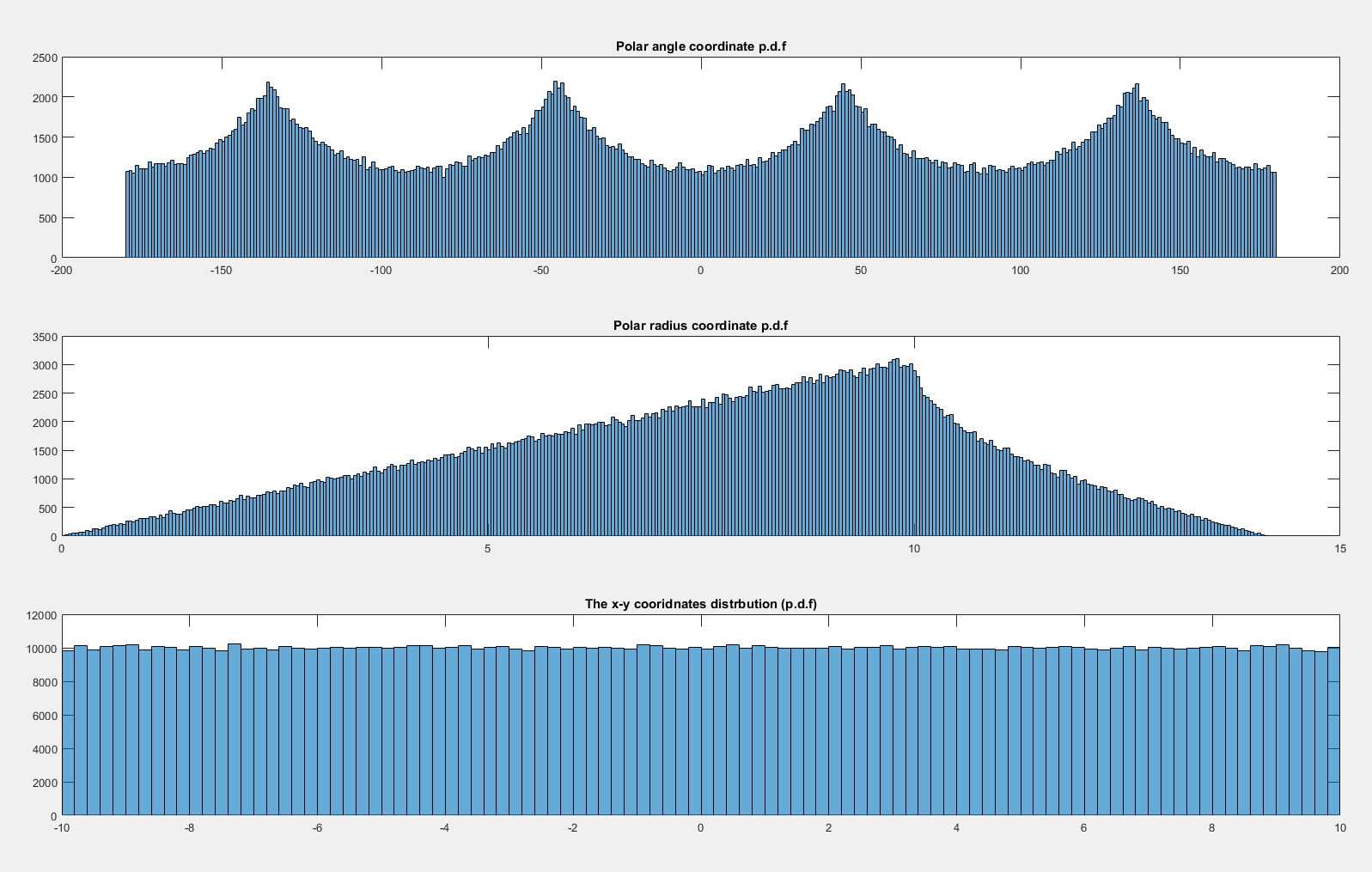
Thus, the radius, $\rho = \sqrt{x^2 + y^2}$, isn't uniformly distributed as implied by $\rho$'s p.d.f.

Nonetheless I would expect $\theta = \arctan{\frac{y}{x}}$ to be almost uniform, excluding artifacts due to the 4 leftovers at the edges:

enter image description here

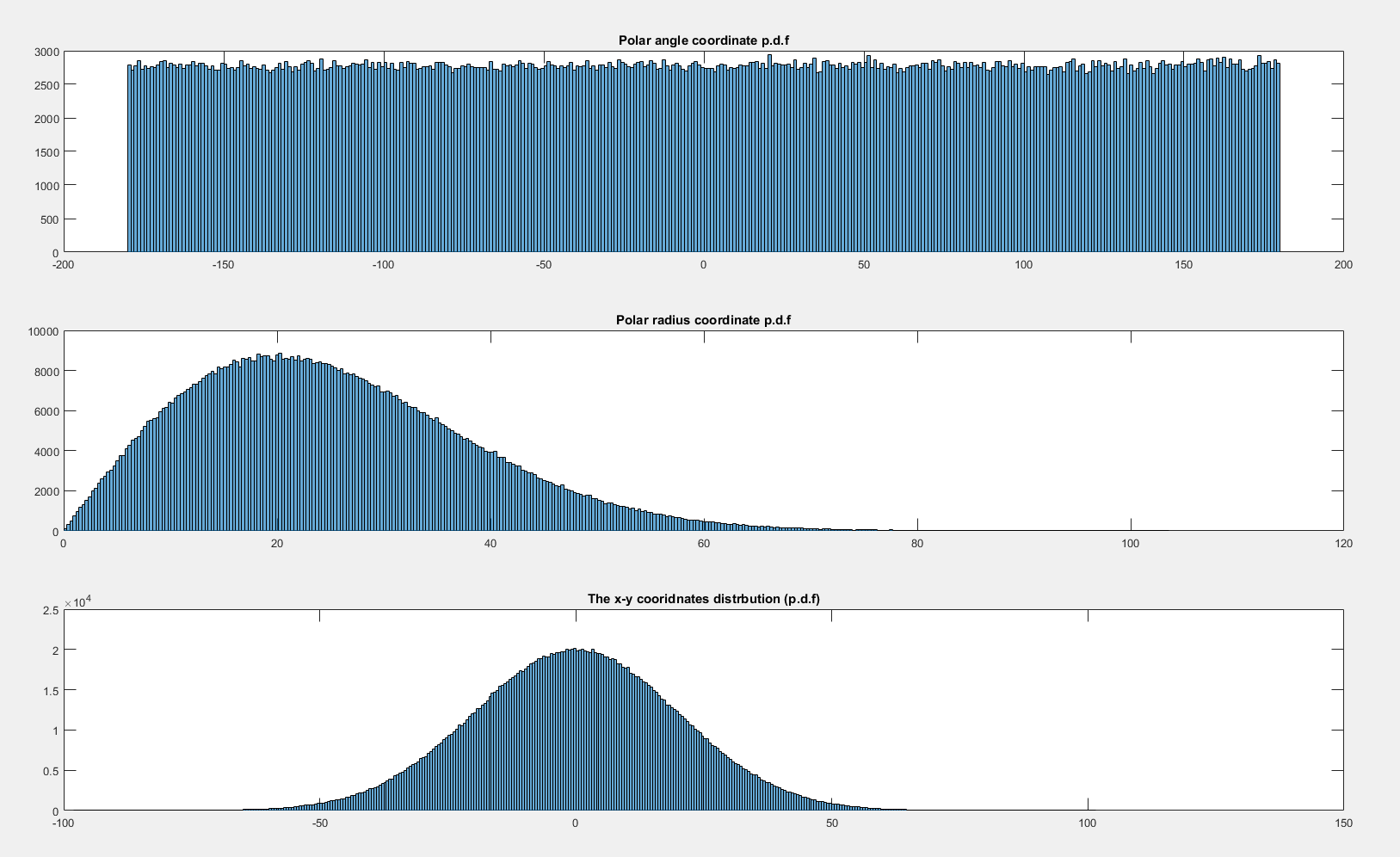
Following are the grafically calculated probability density functions of $\theta$ and $\rho$: enter image description here

Now if I let $x,y$ be distributed s.t. $x,y \sim N(0,20^2)\times N(0,20^2)$ then $\theta$ seems uniformly distributed:

enter image description here

Why $\theta$ isn't uniform when $(x,y) \sim U(-10,10) \times U(-10,10)$ and is uniform when $x,y \sim N(0,20^2)\times N(0,20^2)$?

The Matlab code I used:

number_of_points = 100000;
rng('shuffle')

a = -10;
b = 10;
r = (b-a).*randn(2,number_of_points);
r = reshape(r, [2,number_of_points]);
I = eye(2);
e1 = I(:,1); e2 = I(:,2);
theta = inf*ones(1,number_of_points);
rho = inf*ones(1,number_of_points);

for i=1:length(r(1,:))
    x = r(:,i);
    [theta(i),rho(i)] = cart2pol(x(1),x(2));        
end

figure
M=3;N=1; bins = 360;
subplot(M,N,1); 
histogram(rad2deg(theta), bins)
title('Polar angle coordinate p.d.f');

subplot(M,N,2); 
histogram(rho, bins);
title('Polar radius coordinate p.d.f');

subplot(M,N,3); 
histogram(r(:));
title('The x-y cooridnates distrbution (p.d.f)');

Substituting the 3rd line: r = (b-a).*randn(2,number_of_points); with r = (b-a).*randn(2,number_of_points) +a ; will change the distribution of $(x,y)$ from normal to uniform.

$\endgroup$
2
  • 5
    $\begingroup$ The question looks prettier and prettier with every edit and the title of the question is clearer and more concise. Well done @0x90. $\endgroup$ Commented Jan 4, 2017 at 9:20
  • 3
    $\begingroup$ +1. It's interesting that the normal distribution is the only one that leads to uniformly distributed angles (i.e. to a rotational symmetric 2D distribution), see stats.stackexchange.com/a/255417/28666. $\endgroup$
    – amoeba
    Commented Jan 10, 2017 at 7:05

3 Answers 3

13
$\begingroup$

You're referring to a transformation from a pair of independent variates $(X,Y)$ to the polar representation $(R,\theta)$ (radius and angle), and then looking at the marginal distribution of $\theta$.

I'm going to offer a somewhat intuitive explanation (though a mathematical derivation of the density does essentially what I describe informally).

Note that if you scale the two variables, X and Y by some common scale (e.g. go from U(-1,1) to U(-10,10) or from N(0,1) to N(0,20) on both variables at the same time) that makes no difference to the distribution of the angle (it only affects the scale of the distribution of the radius). So let's just consider the unit cases.

First consider what's going on with the uniform case. Note that the distribution is uniform over the unit square, so that the probability density in a region that's contained within $[-1,1]^2$ is proportional to the area of the region. Specifically, look at the density associated with an element of angle, $d\theta$ near the horizontal (near angle $\theta=0$) and on the diagonal (near angle $\theta=\pi/4$):
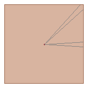
enter image description here

Clearly the probability element $df_\theta$ (i.e. area) corresponding to an element of angle ($d\theta$) is larger when the angle is near one of the diagonals. Indeed consider inscribing a circle inside the square; the area spanned by a given tiny angle within the circle is constant, and then the part outside the circle grows as we approach the diagonal, where it at its maximum.

This completely accounts for the pattern you see in the simulations.

Indeed, we can see that the density must be proportional to the length of the segment from the center of the square to its edge; simple trigonometry is sufficient to derive the density from there and then it's easy to find the constant required to make the density integrate to 1.

[Edit: added this next bit to discuss the radius, since the question has changed since my original answer.]

Note that if we had a uniform distribution over the unit circle (i.e. the one we inscribed in the square before) then the density of the radius for that would be proportional to the radius (consider the area of a small annular element of width $dr$ at radius $r$ - i.e. between $r$ and $r+dr$ - has area proportional to $r$). Then as we pass outside the circle, new annular regions with larger radius only get density contributions from the part in the square, so the density decreases (initially quite rapidly, then more slowly) between $1$ and $\sqrt 2$. (Again, fairly simple geometrical notions are sufficient to get the functional form of the density if it is needed.)


By contrast, if the joint distribution is rotationally symmetric about the origin then the probability element at some angle doesn't depend on the angle (this is essentially a tautology!). The bivariate distribution of two independent standard Gaussians is rotationally symmetric about the origin:
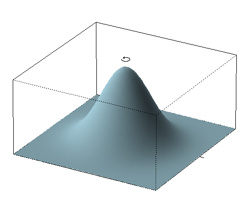
enter image description here

(code for this image based on Elan Cohen's code here but there's a nice alternative here, and something between the two here)

Consequently the volume contained in some angle $d\theta$ is the same for every $\theta$, so the density associated with the angle is uniform on $[0,2\pi)$.

[The polar trick typically used for integrating the normal density over the real line can be used to figure out that the density of the squared radius is negative exponential, and from there the density of the radius is simple to identify by a simple transformation argument from the distribution function]
$\endgroup$
4
  • 4
    $\begingroup$ The four spikes in the distribution of $\theta$ are indeed due to the four corners of the square $(-10,10)^2$. Note that any spherically symmetric distribution will lead to the Uniform distribution on $\theta$, starting with the Uniforms on spheres and circles centred at $(0,0)$. $\endgroup$
    – Xi'an
    Commented Jan 4, 2017 at 6:33
  • 3
    $\begingroup$ +1. It's interesting that the normal distribution is the only one that leads to a rotational symmetric 2D distribution, see stats.stackexchange.com/a/255417/28666. This was surprising to me. $\endgroup$
    – amoeba
    Commented Jan 10, 2017 at 7:04
  • 3
    $\begingroup$ @amoeba Yeah, it's the only circular symmetric distribution that's the product of independent margins. $\endgroup$
    – Glen_b
    Commented Jan 10, 2017 at 10:53
  • 2
    $\begingroup$ I think it's pretty amazing. Consider mentioning it in your answer! $\endgroup$
    – amoeba
    Commented Jan 10, 2017 at 11:06
8
$\begingroup$

To complete the fairly good answers given by Glen and Michael, I'll just compute the density of $\theta$ when the distribution of $(X,Y)$ is uniform on the square $[-1,1]\times[-1,1]$. This uniform density is $1 \over 4$ on this square, $0$ elsewhere -- that is, the probability of sampling a point in a given region of the square is $1 \over 4$ the area of this region.

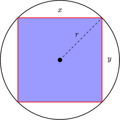
The region of interest for our question is the red sector on this drawing: square with a shaded sector

It’s a triangle delimited by the angle $\theta$ and $\theta + d\theta$. The probability of sampling a point in this triangle is the probability of sampling a value between $\theta$ and $\theta + d\theta$ — which is the density of $\theta$.

I’ll make the computation for $\theta\in \left[ -{\pi \over 4}, {\pi\over 4}\right]$ -- the whole density can be obtained by extending it by $\pi\over 2$ periodicity.

Elementary trigonometry show that the lower side has length $1\over \cos\theta$. The upper size has length $$ {1\over \cos(\theta + d\theta)} = {1\over \cos\theta} + {\sin \theta \over \cos^2\theta} d\theta.$$ (We’ll see that the precise value of the derivative doesn’t really matter here!)

Now the area of a triangle with two sides of lengthes $a$ and $b$ forming an angle $\alpha$ is ${1\over 2}ab\sin\alpha$, hence in our case $$ {1\over 2} \left({1\over \cos\theta} \right) \left({1\over \cos\theta} + {\sin \theta \over \cos^2\theta} d\theta\right) \sin d\theta = {d\theta \over 2\cos^2 \theta}$$ (we neglect higher powers of $d\theta$ and use $\sin d \theta= d\theta$).

Thus the density of $\theta$ is $$ {1\over 8 \cos^2 \theta}$$ for $\theta$ in $\left[-{\pi\over 4},{\pi\over 4}\right]$, and is $\pi\over 2$ periodic.

Verification:

x <- runif(1e6, -1, 1)
y <- runif(1e6, -1, 1)
hist( atan2(y,x), freq=FALSE, breaks=100)
theta <- seq(-pi, pi, length=500)
lines(theta, 0.125/cos((theta + pi/4)%%(pi/2) - pi/4)**2, col="red" )

histogramm + density

$\endgroup$
6
$\begingroup$

I will answer the question about the normal case leading to the uniform distribution. It is well known that if $X$ and $Y$ are independent and normally distributed the contours of constant probability density is a circle in the $x-y$ plane. The radius $R= \sqrt{X^2+ Y^2}$ has the Rayleigh distribution. For a good discussion of this, see the Wikipedia article titled Rayleigh distribution.

Now let us look at the random variables $X$ and $Y$ using polar coordinates.

$X = r\cos(\theta)$, $Y = r \sin(\theta)$. note that $X^2 +Y^2= r^2$. If $\theta$ is uniform on $(0,2 \pi)$ and $r$ has a Rayleigh distribution $X$ and $Y$ will be independent normals each with $0$ mean and common variance. The converse is also true. The proof of the converse is what I think the OP wants as the answer to the second part of the question.

Here is a sketch of the proof. Without loss of generality, we can assume that $X$ is distributed $N(0,1)$ and $Y$ is distributed $N(0,1)$ and independent of each other.

Then the joint density $f(x,y) = (1/2 \pi)\exp[(-[x^2 +y^2])/2]$. Use the transformation to polar coordinates to get $g(r, \theta)$. Since $x = r \sin(\theta)$ and $y = r \cos(\theta)$. So $r= \sqrt{x^2 + y^2}$ and $\theta = \arctan(x/y)$. Compute the Jacobian of the transformation and make the appropriate substitution into $f(x,y)$. as a result $g(r, \theta)$ will be $r \exp[(-r^2)/(2 \pi)]$ for $r\geq0$ and $0\leq\theta\leq 2 \pi$. This shows that $r$ and theta are independent with $r$ having a Rayleigh distribution and theta has the constant density $1/(2 \pi)$.

$\endgroup$
7
  • $\begingroup$ What it means is that if you look at the height of the bivariate density at a fixed radial distance from the center (in this case the origin) it will be the same value on all points on that circle. $\endgroup$ Commented Jan 4, 2017 at 6:55
  • $\begingroup$ math.hkbu.edu.hk/~hpeng/stat3710/Lecture_note3.pdf $\endgroup$
    – 0x90
    Commented Jan 4, 2017 at 7:00
  • $\begingroup$ @0x90 Yes your link shows one way to see this is to look at the quadratic form in the exponent of the density. So in general for the bivariate normal setting that exponent to a constant defines the contours of constant density and that equation is one of an ellipse. in the special case when the covariance matrix is a scaled identity matirix the ellipse simplifies to a circle. $\endgroup$ Commented Jan 4, 2017 at 7:11
  • 2
    $\begingroup$ I think there is an easier way to see the uniformity: for independent normal $X,Y$ with mean $0$, it's easy to show that their ratio is $\operatorname{Cauchy}(0,1)$. Since CDF of Cauchy is simply scaling and translation of $\arctan$, by probability integral transform $\arctan(X/Y)$ is simply a shifted and scaled standard uniform random variable. $\endgroup$
    – Francis
    Commented Jan 4, 2017 at 15:39
  • 1
    $\begingroup$ @Francis Mostly I am appreciative of your thorough editing of all my equations. I also want to say that your comment above definitely shows an imaginative approach to solving the uniformity issue with theta. I am sure some will agree that it is easier. $\endgroup$ Commented Jan 4, 2017 at 16:01

Your Answer

By clicking “Post Your Answer”, you agree to our terms of service and acknowledge you have read our privacy policy.

Not the answer you're looking for? Browse other questions tagged or ask your own question.