16
$\begingroup$

Define the lasso estimate $$\hat\beta^\lambda = \arg\min_{\beta \in \mathbb{R}^p} \frac{1}{2n} \|y - X \beta\|_2^2 + \lambda \|\beta\|_1,$$ where the $i^{th}$ row $x_i \in \mathbb{R}^p$ of the design matrix $X \in \mathbb{R}^{n \times p}$ is a vector of covariates for explaining the stochastic response $y_i$ (for $i=1, \dots n$).

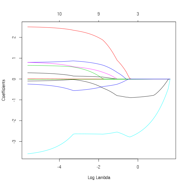
We know that for $\lambda \geq \frac{1}{n} \|X^T y\|_\infty$, the lasso estimate $\hat\beta^\lambda = 0$. (See, for instance, Lasso and Ridge tuning parameter scope.) In other notation, this is expressing that $\lambda_\max = \frac{1}{n} \|X^T y\|_\infty$. Notice that $\lambda_\mathrm{max} = \sup_{\hat\beta^\lambda \ne 0} \lambda.$ We can see this visually with the following image displaying the lasso solution path:

lasso solution path

Notice that on the far right hand side of the plot, all of the coefficients are zero. This happens at the point $\lambda_\mathrm{max}$ described above.

From this plot, we also notice that on the far left side, all of the coefficient are nonzero: what is the value of $\lambda$ at which any component of $\hat\beta^\lambda$ is initially zero? That is, what is $$\lambda_\textrm{min} = \min_{\exists j \, \mathrm{ s.t. } \, \hat\beta_j = 0} \lambda$$ equal to, as a function of $X$ and $y$? I'm interested in a closed form solution. In particular, I'm not interested in an algorithmic solution, such as, for instance, suggesting that LARS could find the knot through computation.

Despite my interests, it seems like $\lambda_\mathrm{min}$ may not be available in closed form, since, otherwise, lasso computational packages would likely take advantage of it when determining the tuning parameter depth during cross validation. In light of this, I'm interested in anything that can be theoretically shown about $\lambda_\mathrm{min}$ and (still) particularly interested in a closed form.

$\endgroup$
15
  • $\begingroup$ This is stated and proven in the glmnet paper: web.stanford.edu/~hastie/Papers/glmnet.pdf $\endgroup$ Commented Jul 6, 2017 at 4:59
  • $\begingroup$ @MatthewDrury Thanks for sharing this! However, this paper doesn't seem to share what you seem to suggest they do. In particular, notice that my $\lambda_\max$ is their $\lambda_\min$. $\endgroup$
    – user795305
    Commented Jul 6, 2017 at 12:06
  • $\begingroup$ Are you sure we need [tuning-parameter] tag? $\endgroup$
    – amoeba
    Commented Jul 6, 2017 at 12:47
  • 1
    $\begingroup$ you a right, a closed form for the lasso solution does in general not exist (see stats.stackexchange.com/questions/174003/…). however, lars at least tells you whats going on and under which exact conditions/at which time you can add/delete a variable. i think something like this is the best you can get. $\endgroup$
    – chRrr
    Commented Jul 7, 2017 at 8:14
  • 1
    $\begingroup$ @chRrr I'm not sure that's completely fair to say: we know that $\hat\beta^\lambda = 0$ for $\lambda \geq \frac{1}{n} \|X^t y\|_\infty$. That is, in the extreme case of the solution being 0, we have a closed form. I'm asking if similar is true in the extreme case of the lasso estimate being dense (ie no zeros). Indeed, I'm not even interested in the exact entries of $\hat\beta_\lambda$---just whether they're zero or not. $\endgroup$
    – user795305
    Commented Jul 7, 2017 at 12:24

2 Answers 2

24
+50
$\begingroup$

The lasso estimate described in the question is the lagrange multiplier equivalent of the following optimization problem:

$${\text{minimize } f(\beta) \text{ subject to } g(\beta) \leq t}$$

$$\begin{align} f(\beta) &= \frac{1}{2n} \vert\vert y-X\beta \vert\vert_2^2 \\ g(\beta) &= \vert\vert \beta \vert\vert_1 \end{align}$$

This optimizazion has a geometric representation of finding the point of contact between a multidimensional sphere and a polytope (spanned by the vectors of X). The surface of the polytope represents $g(\beta)$. The square of the radius of the sphere represents the function $f(\beta)$ and is minimized when the surfaces contact.

The images below provides a graphical explanation. The images made use of the following simple problem with vectors of length 3 (for simplicity in order to be able to make a drawing):

$$\begin{bmatrix} y_1 \\ y_2 \\ y_3\\ \end{bmatrix} = \begin{bmatrix} 1.4 \\ 1.84 \\ 0.32\\ \end{bmatrix} = \beta_1 \begin{bmatrix} 0.8 \\ 0.6 \\ 0\\ \end{bmatrix} +\beta_2 \begin{bmatrix} 0 \\ 0.6 \\ 0.8\\ \end{bmatrix} +\beta_3 \begin{bmatrix} 0.6 \\ 0.64 \\ -0.48\\ \end{bmatrix} + \begin{bmatrix} \epsilon_1 \\ \epsilon_2 \\ \epsilon_3\\ \end{bmatrix} $$ and we minimize $\epsilon_1^2+\epsilon_2^2+\epsilon_3^2$ with the constraint $abs(\beta_1)+abs(\beta_2)+abs(\beta_3) \leq t$

The images show:

  • The red surface depicts the constraint, a polytope spanned by X.
  • And the green surface depicts the minimalized surface, a sphere.
  • The blue line shows the lasso path, the solutions that we find as we change $t$ or $\lambda$.
  • The green vector shows the OLS solution $\hat{y}$ (which was chosen as $\beta_1=\beta_2=\beta_3=1$ or $\hat{y} = x_1 + x_2 + x_3$.
  • The three black vectors are $x_1 = (0.8,0.6,0)$, $x_2 = (0,0.6,0.8)$ and $x_3 = (0.6,0.64,-0.48)$.

We show three images:

  1. In the first image only a point of the polytope is touching the sphere. This image demonstrates very well why the lasso solution is not just a multiple of the OLS solution. The direction of the OLS solution adds stronger to the sum $\vert \beta \vert_1$. In this case only a single $\beta_i$ is non-zero.
  2. In the second image a ridge of the polytope is touching the sphere (in higher dimensions we get higher dimensional analogues). In this case multiple $\beta_i$ are non-zero.
  3. In the third image a facet tof the polytope is touching the sphere. In this case all the $\beta_i$ are nonzero.

The range of $t$ or $\lambda$ for which we have the first and third cases can be easily calculated due to their simple geometric representation.

##Case 1: Only a single $\beta_i$ non-zero##

The non-zero $\beta_i$ is the one for which the associated vector $x_i$ has the highest absolute value of the covariance with $\hat{y}$ (this is the point of the parrallelotope which closest to the OLS solution). We can calculate the Lagrange multiplier $\lambda_{max}$ below which we have at least a non-zero $\beta$ by taking the derivative with $\pm\beta_i$ (the sign depending on whether we increase the $\beta_i$ in negative or positive direction ):

$$\frac{\partial ( \frac{1}{2n} \vert \vert y - X\beta \vert \vert_2^2 - \lambda \vert \vert \beta \vert \vert_1 )}{\pm \partial \beta_i} = 0$$

which leads to

$$\lambda_{max} = \frac{ \left( \frac{1}{2n}\frac{\partial ( \vert \vert y - X\beta \vert \vert_2^2}{\pm \partial \beta_i} \right) }{ \left( \frac{ \vert \vert \beta \vert \vert_1 )}{\pm \partial \beta_i}\right)} = \pm \frac{\partial ( \frac{1}{2n} \vert \vert y - X\beta \vert \vert_2^2}{\partial \beta_i} = \pm \frac{1}{n} x_i \cdot y $$

which equals the $\vert \vert X^Ty \vert \vert_\infty$ mentioned in the comments.

where we should notice that this is only true for the special case in which the tip of the polytope is touching the sphere (so this is not a general solution, although generalization is straightforward).

##Case 3: All $\beta_i$ are non-zero.##

In this case that a facet of the polytope is touching the sphere. Then the direction of change of the lasso path is normal to the surface of the particular facet.

The polytope has many facets, with positive and negative contributions of the $x_i$. In the case of the last lasso step, when the lasso solution is close to the ols solution, then the contributions of the $x_i$ must be defined by the sign of the OLS solution. The normal of the facet can be defined by taking the gradient of the function $\vert \vert \beta(r) \vert \vert_1 $, the value of the sum of beta at the point $r$, which is:

$$ n = - \nabla_r ( \vert \vert \beta(r) \vert \vert_1) = -\nabla_r ( \text{sign} (\hat{\beta}) \cdot (X^TX)^{-1}X^Tr ) = -\text{sign} (\hat{\beta}) \cdot (X^TX)^{-1}X^T $$

and the equivalent change of beta for this direction is:

$$ \vec{\beta}_{last} = (X^TX)^{-1}X n = -(X^TX)^{-1}X^T [\text{sign} (\hat{\beta}) \cdot (X^TX)^{-1}X^T]$$

which after some algebraic tricks with shifting the transposes ($A^TB^T = [BA]^T$) and distribution of brackets becomes

$$ \vec{\beta}_{last} = - (X^TX)^{-1} \text{sign} (\hat{\beta}) $$

we normalize this direction:

$$ \vec{\beta}_{last,normalized} = \frac{\vec{\beta}_{last}}{\sum \vec{\beta}_{last} \cdot sign(\hat{\beta})} $$

To find the $\lambda_{min}$ below which all coefficients are non-zero. We only have to calculate back from the OLS solution back to the point where one of the coefficients is zero,

$$ d = min \left( \frac{\hat{\beta}}{\vec{\beta}_{last,normalized}} \right)\qquad \text{with the condition that } \frac{\hat{\beta}}{\vec{\beta}_{last,normalized}} >0$$

,and at this point we evaluate the derivative (as before when we calculate $\lambda_{max}$). We use that for a quadratic function we have $q'(x) = 2 q(1) x$:

$$\lambda_{min} = \frac{d}{n} \vert \vert X \vec{\beta}_{last,normalized} \vert \vert_2^2 $$

##Images##

a point of the polytope is touching the sphere, a single $\beta_i$ is non-zero:
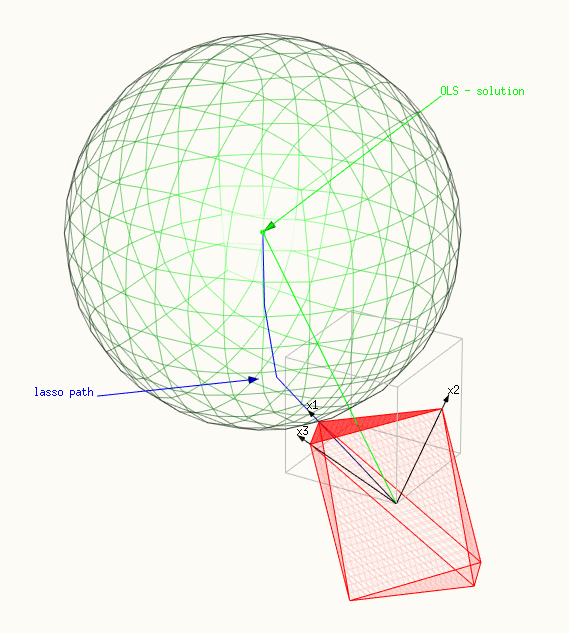
first step of lasso path

a ridge (or differen in multiple dimensions) of the polytope is touching the sphere, many $\beta_i$ are non-zero:
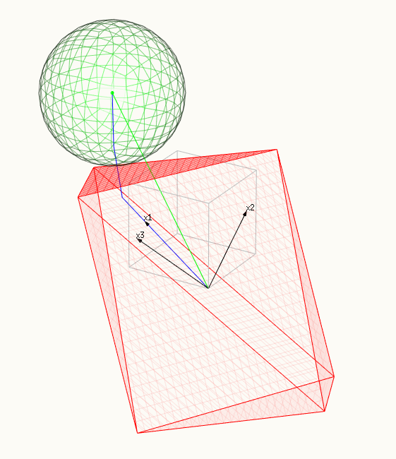
middle of lasso path

a facet of the polytope is touching the sphere, all $\beta_i$ are non-zero:
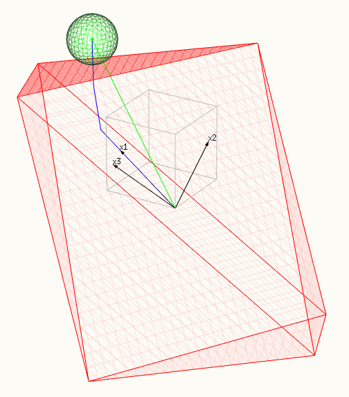
final step of lasso path

##Code example: ##

library(lars)    
data(diabetes)
y <- diabetes$y - mean(diabetes$y)
x <- diabetes$x

# models
lmc <- coef(lm(y~0+x))
modl <- lars(diabetes$x, diabetes$y, type="lasso")

# matrix equation
d_x <- matrix(rep(x[,1],9),length(x[,1])) %*% diag(sign(lmc[-c(1)]/lmc[1]))
x_c = x[,-1]-d_x
y_c = -x[,1]

# solving equation
cof <- coefficients(lm(y_c~0+x_c))
cof <- c(1-sum(cof*sign(lmc[-c(1)]/lmc[1])),cof)

# alternatively the last direction of change in coefficients is found by:
solve(t(x) %*% x) %*% sign(lmc)
  
# solution by lars package
cof_m <-(coefficients(modl)[13,]-coefficients(modl)[12,])

# last step
dist <- x %*% (cof/sum(cof*sign(lmc[])))
#dist_m <- x %*% (cof_m/sum(cof_m*sign(lmc[]))) #for comparison

# calculate back to zero
shrinking_set <- which(-lmc[]/cof>0)  #only the positive values
step_last <- min((-lmc/cof)[shrinking_set])

d_err_d_beta <- step_last*sum(dist^2)

# compare
modl[4] #all computed lambda
d_err_d_beta  # lambda last change
max(t(x) %*% y) # lambda first change
enter code here

note: those last three lines are the most important

> modl[4]            # all computed lambda by algorithm
$lambda
 [1] 949.435260 889.315991 452.900969 316.074053 130.130851  88.782430  68.965221  19.981255   5.477473   5.089179
[11]   2.182250   1.310435

> d_err_d_beta       # lambda last change by calculating only last step
    xhdl 
1.310435 
> max(t(x) %*% y)    # lambda first change by max(x^T y)
[1] 949.4353

(edit notice: this answer had been edited a lot. I have deleted old parts. But left this answer from July 14 which contains a nice explanation of the separation of $y$, $\epsilon$ and $\hat{y}$. The problems that occured in this initial answer have been solved. The final step of the LARS algorithm is easy to find, it is the normal of the polytope defined by the sign of the $\hat{\beta}$) #ANSWER JULI 14 2017#

for $\lambda < \lambda_{max}$ we have at least one non-zero coefficient (and above all are zero)

for $\lambda < \lambda_{min}$ we have all coefficients non-zero (and above at least one coefficient is zero)

finding $\lambda_{max}$

You can use the following steps to determine $\lambda_{max}$ (and this technique will also help for $\lambda_{min}$ although a bit more difficult). For $\lambda>\lambda_{max}$ we have $\hat{\beta}^\lambda$ = 0, as the penalty in the term $\lambda \vert \vert \beta \vert \vert_1$ will be too large, and an increase of $\beta$ does not reduce $(1/2n) \vert \vert y-X \beta \vert \vert ^2_2$ sufficiently to optimize the following expression

(1) \begin{equation}\frac{1}{2n} \vert \vert y-X \beta \vert \vert ^2_2 + \lambda \vert \vert \beta \vert \vert_1 \end{equation}

The basic idea is that at some level of $\lambda$ the increase of $\vert \vert \beta \vert \vert_1$ will cause the term $(1/2n) \vert \vert y-X \beta \vert \vert ^2_2$ to decreases more than the term $\lambda \vert \vert \beta \vert \vert_1$ increases. This point at which the terms are equal can be calculated exactly and at this point the expression (1) can be optimized by an increase of $\beta$ and this is the point below which some terms of $\beta$ are non-zero.

  • Determine the angle, or unit vector $\beta_0$, along which the sum $(y - X\beta)^2$ would decrease most. (in the same way as the first step in the LARS algorithm explained in the very nice article referenced by chRrr) This would relate to the variable(s) $x_i$ that correlates the most with $y$.
  • Calculate the rate of change at which the sum of squares of the error change if you increase the length of the predicted vector $\hat{y}$

$r_1= \frac{1}{2n} \frac{\partial\sum{(y - X\beta_0\cdot s)^2}}{\partial s}$

this is related to the angle between $\vec{\beta_0}$ and $\vec{y}$. The change of the square of the length of the error term $y_{err}$ will be equal to

$\frac{\partial y_{err}^2}{\partial \vert \vert \beta_0 \vert \vert _1} = 2 y_{err} \frac{\partial y_{err}}{\partial \vert \vert \beta_0 \vert \vert _1} = 2 \vert \vert y \vert \vert _2 \vert \vert X\beta_0 \vert \vert _2 cor(\beta_0,y)$

The term $\vert \vert X\beta_0 \vert \vert _2 cor(\beta_0,y)$ is how much the length $y_{err}$ changes as the coefficient $\beta_0$ changes and this includes a multiplication with $X$ (since the larger $X$ the larger the change as the coefficient changes) and a multiplication with the correlation (since only the projection part reduces the length of the error vector).


Then $\lambda_{max}$ is equal to this rate of change and $\lambda_{max} = \frac{1}{2n} \frac{\partial\sum{(y - X\beta_0\cdot s)^2}}{\partial s} = \frac{1}{2n} 2 \vert \vert y \vert \vert _2 \vert \vert x \vert \vert _2 corr(\beta_0,y) = \frac{1}{n} \vert \vert X\beta_0 \cdot y \vert \vert _2 $

Where $\beta_0$ is the unit vector that corresponds to the angle in the first step of the LARS algorithm.

If $k$ is the number of vectors that share the maximum correlation then we have

$\lambda_{max} = \frac{\sqrt{k}}{n} \vert \vert X^T y\vert \vert_\infty $


In other words. LARS gives you the initial decline of the SSE as you increase the length of the vector $\beta$ and this is then equal to your $\lambda_{max}$


##Graphical example##

The image below explains the concept how the LARS algorithm can help in finding $\lambda_{max}$. (and also hints how we can find $\lambda_{min}$)

  • In the image we see schematically the fitting of the vector $y$ by the vectors $x_1$ and $x_2$.
  • The dotted gray vectors depict the OLS solution with $y_{\perp}$ the part of $y$ that is perpendicular (the error) to the span of the vectors $x_1$ and $x_2$ (and the perpendicular vector is the shortest distance and the smallest sum of squares)
  • the gray lines are iso-lines for which $\vert \vert \beta \vert \vert_1$ is constant
  • The vectors $\beta_0$ and $\beta_1$ depict the path that is being followed in a LARS regression.
  • the blue lines and green lines are the vectors that depict the error term as the LARS regression algorithm is followed. the length of these lines is the SSE and when they reach the perpendicular vector $y_{\perp}$ you have the least sum of squares

Now, initially the path is followed along the vector $x_i$ that has the highest correlation with $y$. For this vector the change of the $\sqrt{SSE}$ as function of the change of $\vert \vert \beta \vert \vert$ is largest (namely equal to the correlation of that vector $x_i$ and $y$). While you follow the path this change of $\sqrt{SSE}$/$\vert \vert \beta \vert \vert$ decreases until a path along a combination of two vectors becomes more efficient, and so on. Notice that the ratio of the change $\sqrt{SSE}$ and change $\vert \vert \beta \vert \vert$ is a monotonously decreasing function. Therefore, the solution for $\lambda_{max}$ must be at the origin.

graphical example of LARS procedure

finding $\lambda_{min} $

The above illustration also shows how we can find $\lambda_{min}$ the point at which all of the coefficients are non zero. This occurs in the last step of the LARS procedure.

We can find this points with similar steps. We can determine the angle of the last step and the pre-last step and determine the point where these steps turn from the one into the other. This point is then used to calculate $\lambda_{min}$.

The expression is a bit more awkard since you do not calculate starting from zero. Actually, a solution may not exist. The vector along which the final step is made is in the direction of $X^T \cdot sign$ in which $sign$ is a vector with 1's and -1's depending on the direction of the change for the coefficient in the last step. This direction can be calculated if you know the result of the pre-last step (and could be achieved by itteration towards the first step but such a huge calculation does not seem to be what we want). I do not seem to find out if we can see directly what the sign is of the change of the coefficients in the last step.

Note note that we can more easily determine the point $\lambda_{opt}$ for which $\beta^\lambda$ is equal to the OLS solution. In the image this is related to the change of the vector $y_{\perp}$ as we move along the slope $\hat{\beta_n}$ (this might be more practical to calculate)

problems with sign changes

The LARS solution is close to the LASSO solution. A difference is in the number of steps. In the above method one would find out the direction of the last change and then go back from the OLS solution untill a coefficient becomes zero. A problem occurs if this point is not a point at which a coefficient is added to the set of active coefficients. It could be also a sign change and the LASSO and LARS solutions may differ in these points.

$\endgroup$
5
  • $\begingroup$ Thanks for including the edits! So far in my reading, I'm stuck just past the "case 1" subsection. The result for $\lambda_\max$ derived there is wrong since it doesn't include an absolute value or a maximum. We know further that there's a mistake since in the derivation, there's a sign mistake, a place where differentiability is wrongly assumed, an "arbitrary choice" of $i$ to differentiate with respect to, and an incorrectly evaluated derivative. To be frank, there isn't one "$=$" sign that's valid. $\endgroup$
    – user795305
    Commented Oct 22, 2017 at 20:26
  • $\begingroup$ I have corrected it with a plus minus sign. The change of the beta can be possitive or negative. Regarding the maximum and "arbitrary choice"... "for which the associated vector $x_i$ has the highest covariance with $\hat{y}$" $\endgroup$ Commented Oct 22, 2017 at 20:55
  • $\begingroup$ Thanks for the update! However, there's still problems. For instance, $\frac{\partial}{\partial \beta_i} \|y - X \beta\|_2^2$ is evaluated incorrectly. $\endgroup$
    – user795305
    Commented Oct 22, 2017 at 21:00
  • $\begingroup$ If $\beta=0$ then $\frac{\partial}{\partial\beta_i} \vert \vert y - X\beta \vert \vert_2^2 $ $$ = \frac{\partial \vert \vert y - X\beta \vert \vert_2}{\partial\beta_i} 2 \vert \vert y - X\beta \vert \vert_2 $$ $$ = \frac{\partial \vert \vert y - s x_i \vert \vert_2}{\partial s} 2 \vert \vert y - X\beta \vert \vert_2 $$ $$ = 2 cor(x_i,y) \vert \vert x_i \vert \vert_2 \vert \vert y \vert \vert_2 $$ $$ = 2 x_i \cdot y $$ this correlation enters the equation because,if s=0 then only the change of $s x_i$ tangent to $y$ is changing the length of the vector $y - s x_i$ $\endgroup$ Commented Oct 22, 2017 at 21:18
  • $\begingroup$ Ah, okay, so there's a limit involved in your argument! (You're using both $\beta = 0$ and that a coefficient is nonzero.) Further, the second equality in the line with $\lambda_\max$ is misleading since the sign could change due to the differentiation of the absolute value. $\endgroup$
    – user795305
    Commented Oct 22, 2017 at 22:00
3
$\begingroup$

The lasso is especially useful when $p>n$, i.e., more parameters than sample size.

If $p>n$ and $X$ has continuous distributions, the least-squares estimate $\hat\beta^{LS}$ that minimizes $\min_{b\in R^p} \|y-Xb\|^2$ is not unique (the affine subspace of least-squares solutions is exactly $\hat\beta^{LS}_0 + \ker(X)$ for any specific solution $\hat\beta^{LS}_0$ and $\ker(X)$ has dimension at least $p-n$).

Also, there exists a least-squares solution with at most $n$ nonzero coordinates and at least $p-n$ zero coordinates. To see this, write $X$ by block as $[X_n|X_{p-n}]$ where $X_n$ is a square $n\times n$ matrix. If $X$ has continuous distribution then $X_n$ is invertible with probability one and $\hat b$ in $R^p$ defined by $X_n^{-1}y$ on the first $n$ coordinates and 0 on the last $(p-n)$ coordinates is a least-squares solution with at least $p-n$ zero entries.

So with probability one, when $p>n$, your $\lambda_{min}$ is equal to 0.

$\endgroup$

Your Answer

By clicking “Post Your Answer”, you agree to our terms of service and acknowledge you have read our privacy policy.

Not the answer you're looking for? Browse other questions tagged or ask your own question.