2
$\begingroup$

I'm trying to estimate how many people participated in a game competition and what my percentile score is based on some public data provided by the host.

The data I have is:

  • Top 50 leaderboard (Let's say the 50th player scored 940.6)
  • top 5th (699.0), 20th(475.3), 40th(214.8) and 70th(107.0) percentile score
  • A (not that clear) curveThe curve Showing how many player have achieved a certain score (X axis is only partially annotated.)

(1) Assuming that the final score distribution is a normal distribution, is it possible to estimate the whole distribution?

  • Giving a score, is it possible to estimate the percentile score?
  • Is it possible to estimate the total entries?

(2) This curve doesn't look like a trivial normal distribution. What's the best guess of this distribution? Can it be two distributions added up? If this is the case, is it possible to separate them just using these data we have?

Edit: I'll give a bit more details how this data is formed. Each player plays in a succession of 3-player match which yields a pre-adjustment zero-sum result (ex. +50, +5, -55 or +50, -15, -35). The final score of a player is generated by his or her best performance summed up in any consecutive 8 games, adding a bonus +60 to each game played (Which means that when a player didn't finish 8 games s/he still qualifies but get less bonus score).

A good simplification is that 3 players play in a poker-style game and got their earnings/lost at the end of the game summed up with an additional bonus/penalty based on their positions. Although players only carry certain chips into a game and when any one depleted their chips or had certain rounds finished the game concludes, negative chips do carry over so scores can be arbitrary large but 99% of the game won't have anything over +/-80. Players got randomly matched.

The game is actually 3 players japanese riichi mahjong. (https://en.wikipedia.org/wiki/Japanese_Mahjong)

Example 1: -50 +50 +50 +50 +50 +50 +50 +50 +50 => Total +400 (Best possible sum at Games 2-9; 1-8 only yields +300 and are not selected) +480 (Finished at least 8 games) = +880

Example 2: -50 +50 => Total +0 (Games 1-2) + 120(Finished 2 games) = +120

Players play minimum 1 game to qualify. The best guess to distribution of how many games a player played is a binomial distribution.

$\endgroup$
7
  • $\begingroup$ What is this curve attempting to display? What is being shown on its axes? It doesn't seem to be even remotely related to a Normal distribution. $\endgroup$
    – whuber
    Commented Nov 7, 2017 at 20:43
  • $\begingroup$ Y axis is "how many players achieved this score", and X axis is "the score". I will add more information to the topic to clarify this. $\endgroup$
    – xxbidiao
    Commented Nov 8, 2017 at 4:11
  • 1
    $\begingroup$ I was worried about that, because the apparent bump in the curve (within the red zone) is incompatible with your description: such a curve necessarily can never increase in height as you move from left to right. $\endgroup$
    – whuber
    Commented Nov 8, 2017 at 14:41
  • $\begingroup$ Can you explain more about the pre-adjustment zero-sum? Is this a random thing for a game? Does a player win one of the three or can there be more? Are scores related to difficulty? Is +50 a maximum score? Are the games between multiple players (making the scoring dependent)? In that case, how are players matched? What does best performance mean? $\endgroup$ Commented Nov 9, 2017 at 16:20
  • $\begingroup$ @MartijnWeterings A good simplification is that 3 players play in a poker-style game and got their earnings/lost at the end of the game summed up with an additional bonus/penalty based on their positions. Although players only carry certain chips into a game and when any one depleted their chips (Edit: Or certain rounds have been finished) the game concludes, negative chips do carry over so scores can be arbitrary large but 99% of the game won't have anything over +/-80. Players got randomly matched. The game is actually 3 players japanese riichi mahjong. $\endgroup$
    – xxbidiao
    Commented Nov 9, 2017 at 17:26

2 Answers 2

3
+50
$\begingroup$

The yellow curve looks like a probability distribution function (and it's shape is not that strange for these type of cases, e.g. scores).

We can check this by extracting the data (for instance https://apps.automeris.io/wpd/)

And we find:

# data for pdf
pdf = matrix(c(50.791730474732, 1.01010101010101, 
               75.2695252679939, 0.869104521478181, 
               101.560490045942, 0.728138970099154, 
               107, 0.708029761628537, 
               145.076569678407, 0.547063282132195, 
               174.087289433384, 0.456649187123919, 
               202.191424196018, 0.376320633594753, 
               215.790199081164, 0.34624963262023, 
               235.735068912711, 0.306185901898, 
               256.5865237366, 0.25603662969666, 
               281.970903522205, 0.236267730907854, 
               302.822358346095, 0.216421489009544, 
               327.300153139357, 0.186536111497827, 
               354.497702909648, 0.166798149952821, 
               384.415007656968, 0.157207604374526, 
               411.612557427259, 0.13746964282952, 
               442.436447166922, 0.137995575974137, 
               475.073506891271, 0.138552446362554, 
               508.617151607963, 0.159326805574891, 
               542.160796324656, 0.159899144585209, 
               571.171516079633, 0.170495150587034, 
               596.555895865237, 0.170928272000248, 
               623.753445635528, 0.151190310455241, 
               653.670750382848, 0.161801785078968, 
               676.335375191424, 0.152087490525469, 
               699.906584992343, 0.142388664593871, 
               722.571209800919, 0.122573359939363, 
               757.021439509954, 0.102959147369561, 
               781.499234303216, 0.0932757900598635, 
               803.257274119449, 0.0734450167834548, 
               824.108728943338, 0.0535987748851454, 
               854.932618683002, 0.0541247080297616, 
               891.196018376723, 0.0345414327037605, 
               931.085758039816, 0.0150200318653611, 
               992.733537519143, 0.0160718981545933, 
               1058.00765696784, 0.00708462883041761),36,byrow=1)

pdf[,2] <- pdf[,2]-pdf[36,2]

# calculating cdf
cdf <- c(0,cumsum((pdf[-1,2]+pdf[-36,2])*(pdf[-1,1]-pdf[-36,1])))

# correction for not knwoing pdf values below 55
cdf <- cdf+50

# plot calculated cdf
plot(pdf[,1],cdf/cdf[36],ylim=c(0,1),log="x",xlab="score",ylab="cdf, percentile")
#points(pdf[,1],cdf/cdf[36],ylim=c(0,1),log="x")

# plot percentiles
points(c(107,214.8,475.3,699),c(0.30,0.60,0.80,0.95),pch=21,bg=2,col=2)
lines(c(940.6,940.6),c(0,1),col=2)
lines(c(823.15,823.15),c(0,1),col=1)

# plot what would have been if we interpret the extracted yellow curve as cdf
lines(pdf[,1],1-pdf[,2],col="yellow",lw=2)

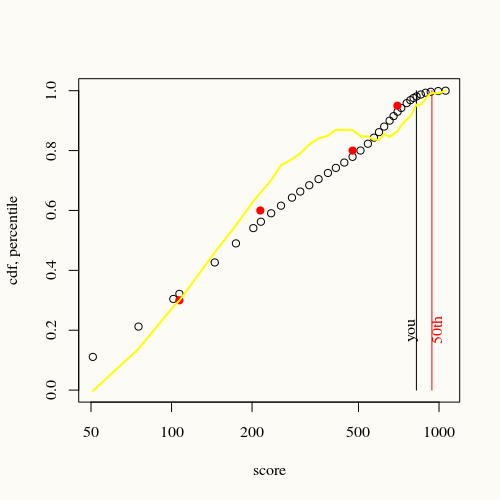
calculated cdf

Which strengthens the believe that the yellow curve in your image was a probability distribution function and not a cumulative distribution function.

There is still a difference between the plotted curve and the given CDF points (at top 5th (699.0), 20th(475.3), 40th(214.8) and 70th(107.0) percentile score) however if we would interpret the yellow curve as a CDF (instead of PDF) then the result is even further off (it has the dip which whuber mentions but also the yellow curve does not match the given percentiles).

In the given diagram you score as 824 at the 98th percentile.

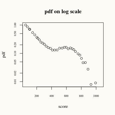
Note: The distribution looks much like an exponential (at least the first part). You see this often in rankings of score boards (for instance: you could do the same with the reputation scores of the users on StackExchange). But also for instance in the wealth distribution of a given population. There are many variations possible, power law, Pareto, etcetera.

So, the assumption of a normal distribution would not be so good.

See the image of log(pdf) log scale of pdf


And now your many questions:

(1)

  • Yes, you can estimate a percentile score based on a given score. This requires an estimate of the CDF. This can be done either based on the yellow curve and the construction of the cdf that I made (reasonably accurate), or based on a exponential distribution and the given percentile scores (less accurate since the distribution is not purely a single exponential distribution, and the bump seems difficult to cast in a simple distribution).

  • Yes, you can estimate the total entries using the previous answer. The top 50th at a score of 940.6 can be estimated by taking an average of the measurement points at 931 and 992, which is roughly 0.9984 and multiplying 50/(1-0.9983579) gives more or less 30k entries. This method is a bit problematic since errors (and we do make them with our simplistic data extraction from the image) tend to blow up for 1/(1-x) when x is close to one.

(2)

  • No definitely not normal distribution.

  • Exponential works but there is a discrepancy between 400 and 600. This is not a-typical for real life distributions.

  • Given your zero sum game mechanism with a bonus that only kicks in after 8 * 60 = 480 this seems to be the possible mechanism with a sum of two distributions.

$\endgroup$
1
  • $\begingroup$ Thanks for the detailed answer! Yes, I have strong belief that the bump around 500~600 is because of the bonus not increasing after +480. By the way even when a player didn't finish 8 games s/he still get discounted bonus point (60 per game) so it's not 0 or 480. $\endgroup$
    – xxbidiao
    Commented Nov 9, 2017 at 17:35
2
$\begingroup$

(1) Yes, given at least two percentile values (plus a normality assumption), you can uncover the whole distribution. First note that the normal distribution is completely characterized by it's mean $\mu$ and standard deviation $\sigma$. I'll use these data points:

5th percentile is 107 20th percentile 214.8

Let Z be standard normal, and X is the underlying (unknown) normal distribution, so that:

$$Z = \frac{X - \mu}{\sigma}$$

The 5th percentile of Z is -1.645 and the 20th percentile is -0.842. Two equations, two unknowns:

$$-1.645 = \frac{107 - \mu}{\sigma}$$ $$-0.842 = \frac{214.8 - \mu}{\sigma}$$

Solving, we get $(\mu, \sigma) = (251.03, 43.02)$.

Edit: Of course, if you use two different percentiles, you'll get different $(\mu, \sigma)$ values, since this distribution is not normal, there's no reason the other data point should agree.

(2) Of course, as you pointed out, this is decidedly nonnormal. Just eyeballing, it could be an exponential or gamma distribution.

$\endgroup$
2

Your Answer

By clicking “Post Your Answer”, you agree to our terms of service and acknowledge you have read our privacy policy.

Not the answer you're looking for? Browse other questions tagged or ask your own question.