Residual plot for mixed model shows obvious trend

Question

I have a paired data set where each subject has been weighed at the onset of an experiment and at the end. I am interested in how growth over time is affected by two crossed factors (feed and enrichment). I have 199 subjects that have all been weighed twice, so there are 398 observations.

My initial model was:

model1<-lmer(va~enrichment*feed*time+(1+time|ID), data=welfare)

Where va = weight, enrichment and feed are factors with two levels (dummy variables), time is also a factor with two levels and ID is subject ID.

One problem with this model, as pointed out here, is that there are only two observations per subject, so I can't have both time and ID in my random specification. This can be solved using Ben Bolker's useful guide where he suggests taking time out of the randoms resulting in a model like this:

model2<-lmer(va~enrichment*feed*time+(1|ID), data=welfare)

Summary:

Linear mixed model fit by REML ['lmerMod']
Formula: va ~ enrichment * feed * time + (1 | ID)
   Data: welfare

REML criterion at convergence: 1559.7

Scaled residuals: 
     Min       1Q   Median       3Q      Max 
-2.82014 -0.38182 -0.04042  0.37271  2.99733 

Random effects:
 Groups   Name        Variance Std.Dev.
 ID       (Intercept) 1.694    1.301   
 Residual             1.706    1.306   
Number of obs: 398, groups:  ID, 199

Fixed effects:
                                     Estimate Std. Error t value
(Intercept)                            3.7146     0.2608  14.244
enrichmentshelter                     -0.2380     0.3688  -0.645
feedhand                              -0.1566     0.3688  -0.425
timeafter                              5.0294     0.2613  19.251
enrichmentshelter:feedhand             0.3612     0.5229   0.691
enrichmentshelter:timeafter           -1.2670     0.3695  -3.429
feedhand:timeafter                     0.2168     0.3695   0.587
enrichmentshelter:feedhand:timeafter   1.4886     0.5238   2.842

Correlation of Fixed Effects:
                (Intr) enrchm fedhnd timftr enrchmntshltr:f enrchmntshltr:t fdhnd:
enrchmntshl     -0.707                                                            
feedhand        -0.707  0.500                                                     
timeafter       -0.501  0.354  0.354                                              
enrchmntshltr:f  0.499 -0.705 -0.705 -0.250                                       
enrchmntshltr:t  0.354 -0.501 -0.250 -0.707  0.353                                
fdhnd:tmftr      0.354 -0.250 -0.501 -0.707  0.353           0.500                
enrchmnts::     -0.250  0.353  0.353  0.499 -0.501          -0.705          -0.705

I find a significant three way interaction (which I expected, enrichment and feed look like they interact):

Models:
m2: va ~ feed * enrichment + enrichment * time + feed * time + (1 | 
m2:     ID)
m1: va ~ enrichment * feed * time + (1 | ID)
   Df    AIC    BIC  logLik deviance  Chisq Chi Df Pr(>Chisq)   
m2  9 1577.8 1613.7 -779.90   1559.8                            
m1 10 1571.7 1611.6 -775.86   1551.7 8.0742      1    0.00449 **
---
Signif. codes:  0 ‘***’ 0.001 ‘**’ 0.01 ‘*’ 0.05 ‘.’ 0.1 ‘ ’ 1

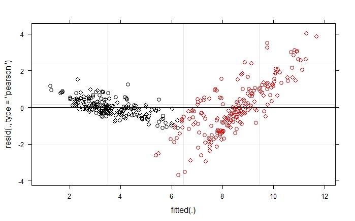
but my residual plot looks like this:

Black dots are time 0 and red dots are time 1. Clearly, the residuals for time 0 and time 1 are nothing alike. I expected them to differ, but also expected to account for this by including time in my error structure.

Does anyone know how I might move forward? A MCMCglmm like this:

mcmcglmm1 <- MCMCglmm(va~enrichment*feed*time,
                      random=~ID,data=welfare,
                      verbose=FALSE)

Spits out pretty similar results to the lme above, but I'm not comfortable with Bayesian modelling and it seems like a lot of work to learn only for this.

 Iterations = 3001:12991
 Thinning interval  = 10
 Sample size  = 1000 

 DIC: 1483.758 

 G-structure:  ~ID

     post.mean l-95% CI u-95% CI eff.samp
ID     1.689    1.171    2.235    862.6

 R-structure:  ~units

      post.mean l-95% CI u-95% CI eff.samp
units     1.731      1.4    2.121    887.7

 Location effects: va ~ enrichment * feed * time 

                                     post.mean l-95% CI u-95% CI eff.samp  pMCMC    
(Intercept)                             3.7159   3.2064   4.2103     1000 <0.001 ***
enrichmentshelter                      -0.2278  -0.8794   0.5591     1000  0.552    
feedhand                               -0.1598  -0.8222   0.5597     1000  0.664    
timeafter                               5.0336   4.5840   5.5456     1000 <0.001 ***
enrichmentshelter:feedhand              0.3534  -0.7479   1.3059     1000  0.502    
enrichmentshelter:timeafter            -1.2810  -1.9796  -0.5750     1127  0.002 ** 
feedhand:timeafter                      0.2179  -0.4005   0.9841     1000  0.566    
enrichmentshelter:feedhand:timeafter    1.4945   0.4772   2.5229     1000  0.010 *  
---
Signif. codes:  0 ‘***’ 0.001 ‘**’ 0.01 ‘*’ 0.05 ‘.’ 0.1 ‘ ’ 1

The simplest solution I can think of, is to only have one observation per subject coded as proportional growth (weightafter-weightbefore)/weightbefore and get rid of random error completely. However, that seems defeatist, and I'd really like to know if I've misspecified the model and whether there's something else I should do.

EDIT:

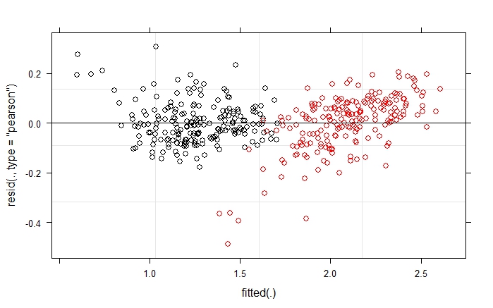
Logged weights produce this plot:

Certainly much better behaved. Hasn't substantially changed results, though they're slightly more similar to the MCMCglmm posted above.

Answer 1

There might be a causality problem with the way you have set up the analysis. If the time 0 weight values were taken before the experimental manipulations (enrichment, feed) were started, then it doesn't make much sense to try to predict the time 0 values from the subsequent experimental manipulations, which is what you implicitly do with your models. What you presumably care about is whether the manipulations affect growth rate, whether that is measured in an absolute, relative, or logarithmic scale.

As you happily have both measurements for all individuals, taking the absolute or relative or logarithmic (my guess is logarithmic will work best) weight change as the fundamental measurement for your linear model should work OK. By doing this you are not really "getting rid of random error completely"; you still have the random error of how much the individuals responded to the manipulations, which seems of primary interest here. Think of this as a generalization of the paired t-test. (You should, however, check that the treatment groups were well balanced with respect to initial time 0 weights.)

Note that this still might not solve your problem with residual magnitudes related to fitted values, however. You might need to explore other transformations of the data for the linear model to achieve that goal, or recognize that the linear model, even with interactions, might not be an adequate representation of the underlying reality.