10
$\begingroup$

I am trying to fit an exponential decay function to y-values that become negative at high x-values, but am unable to configure my nls function correctly.

Aim

I am interested in the slope of the decay function ($\lambda$ according to some sources). How I get this slope is not important, but the model should fit my data as well as possible (i.e. linearizing the problem is acceptable, if the fit is good; see "linearization"). Yet, previous works on this topic have used a following exponential decay function (closed access article by Stedmon et al., equation 3):

$f(y) = a \times exp(-S \times x) + K$

where S is the slope I am interested in, K the correction factor to allow negative values and a the initial value for x (i.e. intercept).

I need to do this in R, as I am writing a function that converts raw measurements of chromophoric dissolved organic matter (CDOM) to values that researchers are interested in.

Example data

Due to the nature of the data, I had to use PasteBin. The example data are available here.

Write dt <- and copy the code fom PasteBin to your R console. I.e.

dt <- structure(list(x = ...

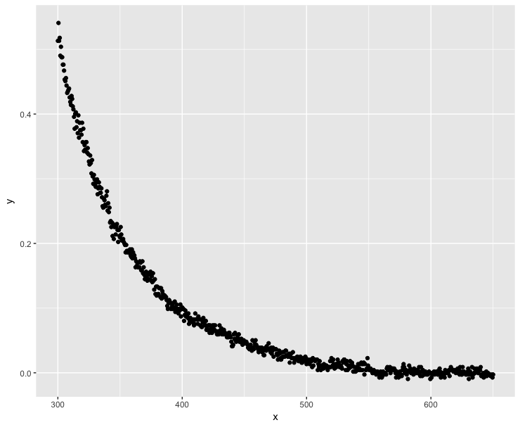
The data look like this:

library(ggplot2)
ggplot(dt, aes(x = x, y = y)) + geom_point()

enter image description here

Negative y values take place when $x > 540 nm$.

Trying to find solution using nls

Initial attempt using nls produces a singularity, which should not be a surprise seeing that I just eyeballed start values for parameters:

nls(y ~ a * exp(-S * x) + K, data = dt, start = list(a = 0.5, S = 0.1, K = -0.1))

# Error in nlsModel(formula, mf, start, wts) : 
#  singular gradient matrix at initial parameter estimates

Following this answer, I can try to make better fitting start parameters to help the nls function:

K0 <- min(dt$y)/2
mod0 <- lm(log(y - K0) ~ x, data = dt) # produces NaNs due to the negative values
start <- list(a = exp(coef(mod0)[1]), S = coef(mod0)[2], K = K0)
nls(y ~ a * exp(-S * x) + K, data = dt, start = start)

# Error in nls(y ~ a * exp(-S * x) + K, data = dt, start = start) : 
#  number of iterations exceeded maximum of 50

The function does not seem to be able to find a solution with the default number of iterations. Let's increase the number of iterations:

nls(y ~ a * exp(-S * x) + K, data = dt, start = start, nls.control(maxiter = 1000))

# Error in nls(y ~ a * exp(-S * x) + K, data = dt, start = start, nls.control(maxiter = 1000)) : 
#  step factor 0.000488281 reduced below 'minFactor' of 0.000976562 

More errors. Chuck it! Let's just force the function to give us a solution:

mod <- nls(y ~ a * exp(-S * x) + K, data = dt, start = start, nls.control(maxiter = 1000, warnOnly = TRUE))
mod.dat <- data.frame(x = dt$x, y = predict(mod, list(wavelength = dt$x)))

ggplot(dt, aes(x = x, y = y)) + geom_point() + 
  geom_line(data = mod.dat, aes(x = x, y = y), color = "red")

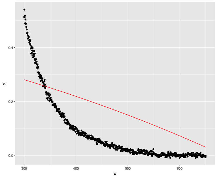
enter image description here

Well, this was definitely not a good solution...

Linearizing the problem

Many people have linearized their exponential decay functions with a success (sources: 1, 2, 3). In this case, we need to make sure that no y value is negative or 0. Let's make the minimum y value as close to 0 as possible within the floating point limits of computers:

K <- abs(min(dt$y)) 
dt$y <- dt$y + K*(1+10^-15)

fit <- lm(log(y) ~ x, data=dt)  
ggplot(dt, aes(x = x, y = y)) + geom_point() + 
geom_line(aes(x=x, y=exp(fit$fitted.values)), color = "red")

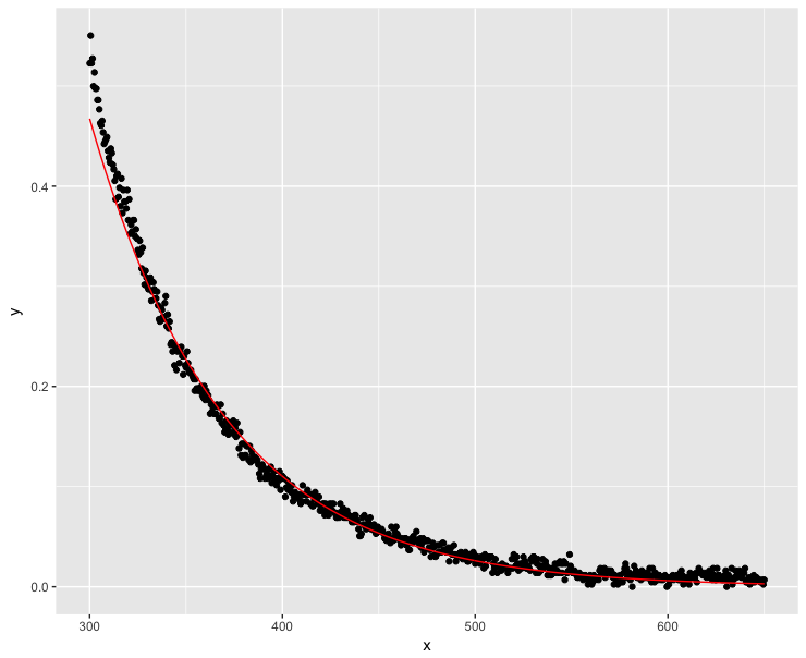
enter image description here

Much better, but the model does not trace y values perfectly at low x values.

Note that the nls function would still not manage to fit the exponential decay:

K0 <- min(dt$y)/2
mod0 <- lm(log(y - K0) ~ x, data = dt) # produces NaNs due to the negative values
start <- list(a = exp(coef(mod0)[1]), S = coef(mod0)[2], K = K0)
nls(y ~ a * exp(-S * x) + K, data = dt, start = start)

# Error in nlsModel(formula, mf, start, wts) : 
#  singular gradient matrix at initial parameter estimates

Do the negative values matter?

The negative values are obviously a measurement error as absorption coefficients cannot be negative. So what if I make the y values generously positive? It is the slope I am interested in. If addition does not affect the slope, I should be settled:

dt$y <- dt$y + 0.1

fit <- lm(log(y) ~ x, data=dt)  
ggplot(dt, aes(x = x, y = y)) + geom_point() + geom_line(aes(x=x, y=exp(fit$fitted.values)), color = "red")
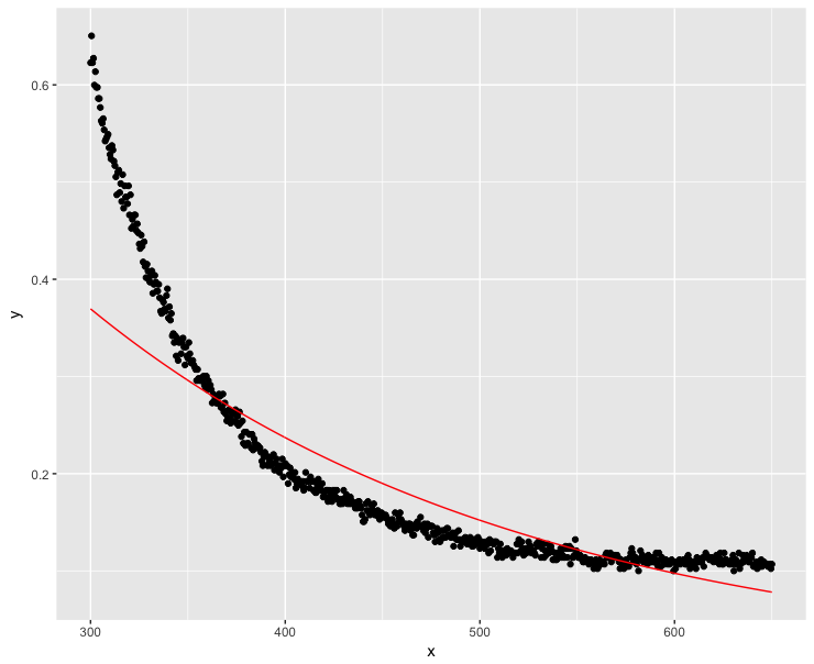
enter image description here Well, this did not go that well...High x values should obviously be as close to zero as possible.

The question

I am obviously doing something wrong here. What is the most accurate way to estimate slope for an exponential decay function fitted on data that have negative y values using R?

$\endgroup$
1
  • 1
    $\begingroup$ nls converged for me using the starting values $a=1, S =0.01, K=-0.0001$. Alternatively, you could use the self-starting function: nls(y~SSasymp(x, Asym, r0, lrc), data = dt). That converges for me too. $\endgroup$ Commented Dec 15, 2017 at 9:59

2 Answers 2

12
$\begingroup$

Use a selfstarting function:

ggplot(dt, aes(x = x, y = y)) + 
  geom_point() +
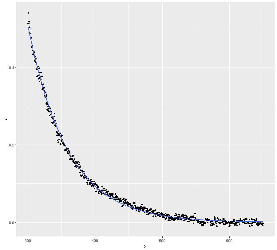
  stat_smooth(method = "nls", formula = y ~ SSasymp(x, Asym, R0, lrc), se = FALSE)

resulting plot

fit <- nls(y ~ SSasymp(x, Asym, R0, lrc), data = dt)
summary(fit)
#Formula: y ~ SSasymp(x, Asym, R0, lrc)
#
#Parameters:
#       Estimate Std. Error  t value Pr(>|t|)    
#Asym -0.0001302  0.0004693   -0.277    0.782    
#R0   77.9103278  2.1432998   36.351   <2e-16 ***
#lrc  -4.0862443  0.0051816 -788.604   <2e-16 ***
#---
#Signif. codes:  0 ‘***’ 0.001 ‘**’ 0.01 ‘*’ 0.05 ‘.’ 0.1 ‘ ’ 1
#
#Residual standard error: 0.007307 on 698 degrees of freedom
#
#Number of iterations to convergence: 0 
#Achieved convergence tolerance: 9.189e-08

exp(coef(fit)[["lrc"]]) #lambda
#[1] 0.01680222

However, I would seriously consider if your domain knowledge doesn't justify setting the asymptote to zero. I believe it does and the above model doesn't disagree (see the standard error / p-value of the coefficient).

ggplot(dt, aes(x = x, y = y)) + 
  geom_point() +
  stat_smooth(method = "nls", formula = y ~ a * exp(-S * x), 
              method.args = list(start = list(a = 78, S = 0.02)), se = FALSE, #starting values obtained from fit above
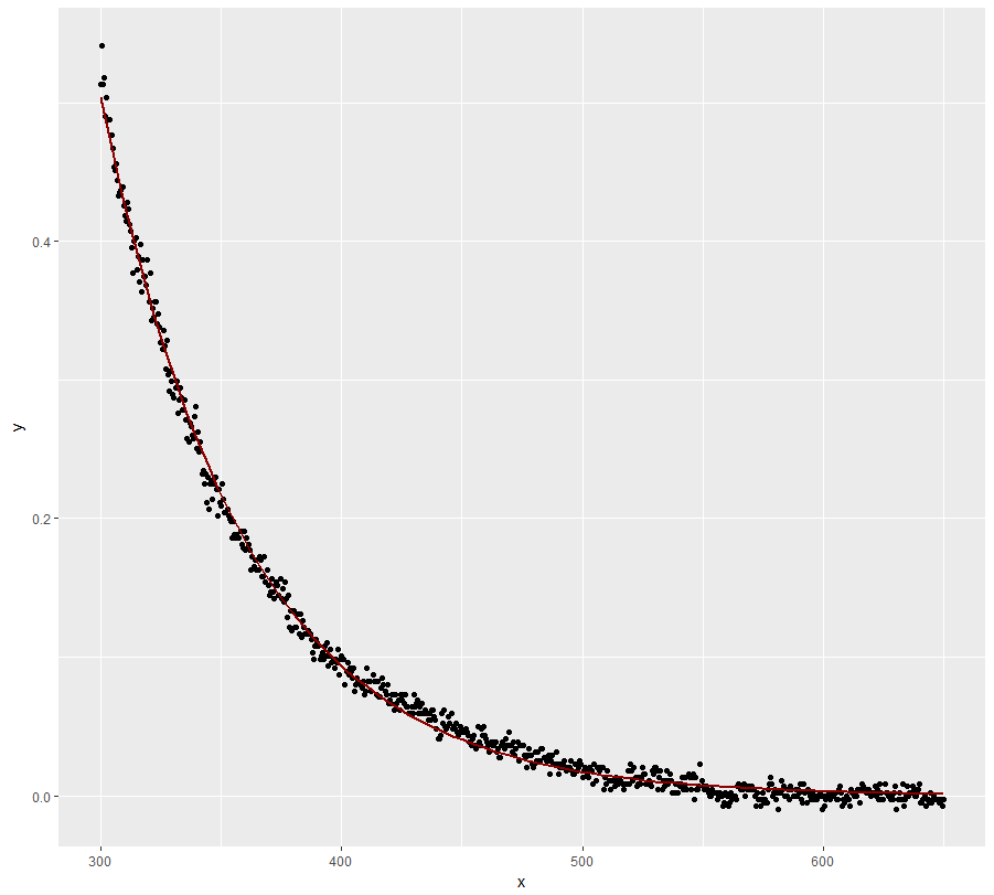
              color = "dark red")

second resulting plot

$\endgroup$
3
  • $\begingroup$ Perfect. I did not know about SSasymp function. Thank you! I believe the researchers want to refer to the article I cited in the question and use the K term, but I will suggest them to modify their equation. I think they want to keep the K, because negative values mean that the instrument did not behave as expected, but they are interested in the slope. Removing the negative asymptote might affect the slope in some instances. $\endgroup$
    – Mikko
    Commented Dec 15, 2017 at 10:37
  • $\begingroup$ @Mikko If you measure absorption and the asymptote gets significantly zero, I would say that you have problems with your calibration or instrument stability. $\endgroup$
    – Roland
    Commented Dec 15, 2017 at 11:12
  • $\begingroup$ The problem often takes place when water is very clear (oceanic water). Some values become below zero. I think we have an instrument that suffers from temperature problems. When it overheats, the values become unstable, but these details should probably not be handled in Crossvalidated. $\endgroup$
    – Mikko
    Commented Dec 15, 2017 at 11:44
3
$\begingroup$

This question has relationships with several other questions

I have three additional remarks regarding some points in this question.

1: Why linearized model does not fit well the large values of $y$

Much better, but the model does not trace y values perfectly at low x values.

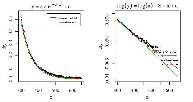
The linearized fit is not minimizing the same residuals. At the logarithmic scale the residuals for smaller values will be larger. The image below shows the comparison by plotting the y-axis on a log scale in the right image:

comparison

When necessary you could add weights to the least squares loss function.

2: Using linearized fit as starting values

After you have obtained estimates with your linearized fit you could have used these as starting point for the non linear fitting.*

# vectors x and y from data
x <- dat$x
y <- dat$y

# linearized fit with zero correction
K <- abs(min(y)) 
dty <- y + K*(1+10^-15)
fit <- lm(log(dty) ~x)  


# old fit that had a singluar gradient matrix error
#         nls(y ~ a * exp(-S * x) + K, 
#                 start = list(a = 0.5, 
#                              S = 0.1, 
#                              K = -0.1))
#

# new fit
fitnls <- nls(y ~ a * exp(-S * x) + K, 
                  start = list(a = exp(fit$coefficients[1]), 
                               S = -fit$coefficients[2], 
                               K = -0.1))
#

3: Using a more general method to obtain the starting point

If you have enough points then you can also obtain the slope without having to worry about asymptotic value and negative values (no computation of a logarithm needed).

You can do this by integrating the data points. Then with $$y = a e^{sx} + k $$ and $$Y = \frac{a}{s} e^{sx} + kx + Const$$ you can use a linear model to obtain the value of $s$ by describing $y$ as a linear combination of the vectors $Y$, $x$ and an intercept:

$$\begin{array}{rccccl}y &=& a e^{sx} + k &=& s(\frac{a}{s} e^{s x} + k x + Const) &- s k x - s Const \\ &&&=& sY &- sk x - s Const \end{array}$$

The advantage of this method (see Tittelbach and Helmrich 1993 "An integration method for the analysis of multiexponential transient signals") is that you can extend it to more than a single exponentially decaying component (adding more integrals).

#
# using Tittelbach Helmrich
#

# integrating with trapezium rule assuming x variable is already ordered
ys <- c(0,cumsum(0.5*diff(x)*(y[-1]+y[-length(y)])))

# getting slope parameter
modth <- lm(y ~ ys + x)
slope <- modth$coefficients[2]

# getting other parameters 
modlm <- lm(y ~ 1 + I(exp(slope*x)))
K <- modlm$coefficients[1]
a <- modlm$coefficients[2]

# fitting with TH start

fitnls2 <- nls(y ~ a * exp(-S * x) + K, 
              start = list(a = a, 
                           S = -slope, 
                           K = K))

Footnote: *This use of the slope in the linearized problem is exactly what what the SSasymp selfstarting function does. It first estimates the asymptote

> stats:::NLSstRtAsymptote.sortedXyData
function (xy) 
{
    in.range <- range(xy$y)
    last.dif <- abs(in.range - xy$y[nrow(xy)])
    if (match(min(last.dif), last.dif) == 2L) 
        in.range[2L] + diff(in.range)/8
    else in.range[1L] - diff(in.range)/8
}

and then the slope by (subtracting the asymptote value and taking the log values)

> stats:::NLSstAsymptotic.sortedXyData
function (xy) 
{
    xy$rt <- NLSstRtAsymptote(xy)
    setNames(coef(nls(y ~ cbind(1, 1 - exp(-exp(lrc) * x)), data = xy, 
        start = list(lrc = log(-coef(lm(log(abs(y - rt)) ~ x, 
            data = xy))[[2L]])), algorithm = "plinear"))[c(2, 
        3, 1)], c("b0", "b1", "lrc"))
}

Note the line start = list(lrc = log(-coef(lm(log(abs(y - rt)) ~ x, data = xy))[[2L]]))

Sidenote: In the special case that $K=0$ you can use

plot(x,y)
mod <- glm(y~x, family = gaussian(link = log), start = c(2,-0.01))
lines(x,exp(predict(mod)),col=2)

which models the observed parameter $y$ as

$$y = exp(X\beta) + \epsilon = exp(\beta_0) \cdot exp(\beta_1 \cdot x) + \epsilon$$

$\endgroup$
8
  • $\begingroup$ What about the case $ {y}_{i} = \exp \left( a x + b \right) + c $ where $ c $ is known? Can this be solved easily with the log transform and Linear Least Squares? In this model I use known c to prevent non positive values. $\endgroup$
    – Royi
    Commented Feb 20, 2021 at 19:07
  • $\begingroup$ @Royi you could linearize this by transforming the output to $z_i = \log(y_i -c)$ for which you have the following relationship $$z_i = \log(y_i -c)= ax+b$$ This is also what happens with the SSasymp starting function which contains the command start = list(lrc = log(-coef(lm(log(abs(y - rt)) ~ x, data = xy))[[2L]])) where this rt is not know as in your case but instead an estimate of the asymptote. $\endgroup$ Commented Feb 20, 2021 at 20:01
  • $\begingroup$ I meant doing so in the context $ c $ is used in order to prevent nonpositive measurements. Hence doing back what you suggested will generate invalid calculation (log() of a negative value). $\endgroup$
    – Royi
    Commented Feb 20, 2021 at 20:50
  • $\begingroup$ @Royi I am not sure how you incorporate $c$ into the model. Do you mean that you artificially introduce it, and bias the model, just in order to prevent nonpositive measurements? $\endgroup$ Commented Feb 20, 2021 at 22:52
  • $\begingroup$ Imagine set of $ {\left\{ {x}_{i}, {y}_{i} \right\}}_{i = 1}^{N} $ from the model $ {y}_{i} = \exp \left( a x + b \right) + {n}_{i} $. Now, due to the additive noise some of the measurements are non positive and even negative. So we choose $ c = \min_{i} {\left\{ {y}_{i} \right\}}_{i = 1}^{N} + 1 $. Then we add it to all measurements. I wonder if that can be still be solved using Linear Least Squares (So we know $ c $ but we can't subtract it before the log() transform). $\endgroup$
    – Royi
    Commented Feb 21, 2021 at 4:54

Your Answer

By clicking “Post Your Answer”, you agree to our terms of service and acknowledge you have read our privacy policy.

Not the answer you're looking for? Browse other questions tagged or ask your own question.