Establishing the Probability Distribution that Governs a Random Process

Question

I have a experiment in which a random event that can occur $N$ times in some set period of time $T$ (where $N \in$ $\mathbb{N_0}$ but is typically less that 10 and never exceeds 100). Here I will refer to a single experiment as a "session", and for a single session we know that the probability of $n$ events occurring in some remaining time $T_{R} = T - t_{i}$ is approximately Poisson distributed, but that this distribution is not "quite right".

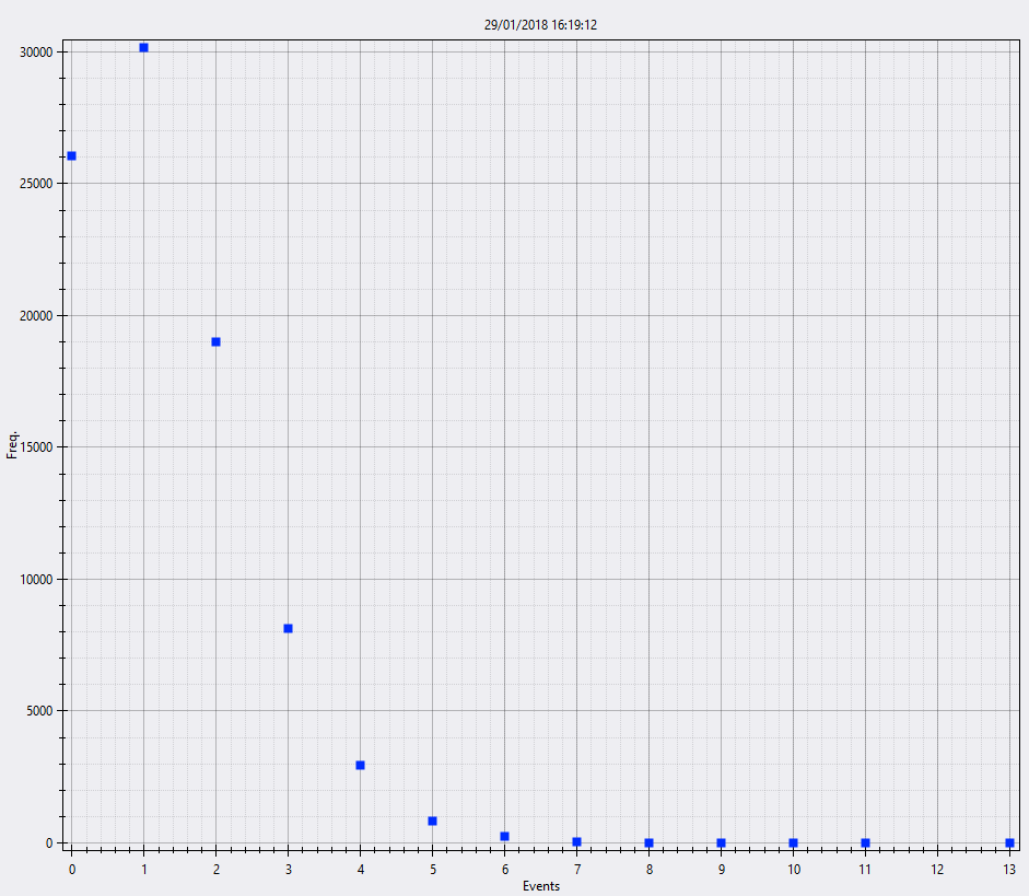
In order to attempt to model the exact way these events are distributed during a "session", I have run ~60,000 sessions, each one with $T = 60$ minutes. From these "sessions" I have gathered the data of how many "event" occurred in the time T. This looks like

We can model the the probability of a number of events occurring in the period $0 \leq t < T$ using a Poisson distribution (which is providing the probability of $n$ events occurring in the time-remaining $t$).

To model the events we let $t$ be the time remaining and $X_t$ be the total number of events to occur in the remaining time $t$. The model implies the estimates $P(X_t \leq c)$. So under our assumption $X_t\sim \operatorname{Poisson}(\lambda_{t})$ we have: $$ P(X_t \leq c) = e^{-\lambda}\sum_{k=0}^c\frac{\lambda_t^k}{k!}\,. $$

This works fairly well during simulation (where we have an implied $\lambda$ from another data source), but we have a belief that the underlying process can be more accurately modeled using a Negative Binomial distribution rather than Poisson. My problem is that I am not a statistician and I don't really know how I can go about extracting the relevant parameters for the Negative Binomial using the data above. I have access to R and am happy to write the necessary code to extract these parameters, I am just unsure about what this process/method of extraction is, can anyone outline this for me?

Better still, if we switch to use Negative Binomial distribution so that we assume now that the probability of a number of events occurring in the period $0 \leq t < T$ is $X_t\sim NB(r, p)$ and we have $$ P(X_{t} \leq c) = p^{r}\sum_{k = 0}^c (1 - p)^{k}\binom{k + r -1}{r - 1}, $$ can anyone provide an R script that can be used to extract my $r$ and $p$?

The data above is:

╔═══════════════╦══════════╗
║ Session Count ║ Events   ║
╠═══════════════╬══════════╣
║  26069        ║ 0        ║
║  30175        ║ 1        ║
║  18997        ║ 2        ║
║  8136         ║ 3        ║
║  2934         ║ 4        ║
║  820          ║ 5        ║
║  250          ║ 6        ║
║  54           ║ 7        ║
║  16           ║ 8        ║
║  4            ║ 9        ║
║  7            ║ 10       ║
║  1            ║ 11       ║
║  0            ║ 12       ║
║  1            ║ 13       ║
╚═══════════════╩══════════╝

Answer 1

Given some data and the general shape of a distribution, it's possible to fit the parameters of that distribution using the principle of Maximum Likelihood Estimation (MLE).

In short, that involves either:

1. using an analytical closed-form solution to fit the parameters exactly
2. solving an optimisation problem to maximise a log-likelihood function, or (more usually) minimise a negative log-likelihood function

Let's first load up your count data in a dataframe:

    count.data <- data.frame(events=0:13, count=c(26069, 30175, 
                            18997, 8136, 2934, 820, 250, 54, 16, 
                            4, 7, 1, 0, 1))

And we'll convert this count data to actual raw observations, for use later:

    raw.data <- rep(count.data$events, count.data$count)

Before going on to the Negative Binomial, let's first fit a Poisson distribution to your data using MLE. This is actually very simple, because the ML estimate of the Poisson parameter $\lambda$ is simply the sample mean:

    poisson.lambda.mle <- mean(raw.data)

We can use this value for $\lambda$ to generate Poisson counts, to compare against yours later:

    fitted.poisson.counts <- dpois(count.data$events, 
              poisson.lambda.mle) * sum(count.data$count)

The Negative Binomial distribution is much more complicated to fit. One reason is that there's no simple analytical expression for its parameters, so it needs to be formulated and solved as an optimisation problem. More importantly, if you parameterise it by an integer $r$, like you are doing, this integer parameter makes the optimisation much harder in R. In fact, I don't know of any native R integer programming functions.

So let's have a quick review of the Negative Binomial: there are actually quite a few ways to parameterise this distribution. The one you've chosen is a "coin-flipping" interpretation based on the number of success/failures, similar to the way the Binomial distribution is taught. There are a few such parameterisations but we actually won't use any of them, for the reasons already discussed.

Instead, the Negative Binomial distribution can be interpreted as a Gamma-mixture of Poisson distributions. This can also be parameterised in a few ways. We will use this one (as described by the R documentation):

An alternative parametrization (often used in ecology) is by the mean mu (see above), and size, the dispersion parameter, where prob = size/(size+mu). The variance is mu + mu^2/size in this parametrization.

The reason we will use this interpreation & parameterisation is because it allows us to use the MASS package's readymade implementation of MLE for the Negative Binomial. Let's get to it:

    library(MASS)
    negbin.fitted.object <- MASS::fitdistr(raw.data, 
              "Negative Binomial")

Once again, we can use these ML estimates for the size and mu parameters to generate counts to compare against yours:

    negbin.size.mle <- negbin.fitted.object$estimate['size']
    negbin.mu.mle <- negbin.fitted.object$estimate['mu']
    fitted.negbin.counts <- dnbinom(count.data$events, 
            size=negbin.size.mle, mu=negbin.mu.mle) * 
              sum(count.data$count)

And that's it. Not only have we fitted Poisson and Negative Binomial distributions to your data, we have prepared counts to compare against yours. Let's print them out together:

    count.comparison <- transform(count.data, 
    fitted.poisson.counts=fitted.poisson.counts, 
      fitted.negbin.counts=fitted.negbin.counts)
    print(round(count.comparison, 0), row.names=FALSE)

which outputs:

     events count fitted.poisson.counts fitted.negbin.counts
          0 26069                 24712                26149
          1 30175                 31234                30178
          2 18997                 19739                18727
          3  8136                  8316                 8291
          4  2934                  2628                 2933
          5   820                   664                  881
          6   250                   140                  233
          7    54                    25                   56
          8    16                     4                   12
          9     4                     1                    3
         10     7                     0                    0
         11     1                     0                    0
         12     0                     0                    0
         13     1                     0                    0

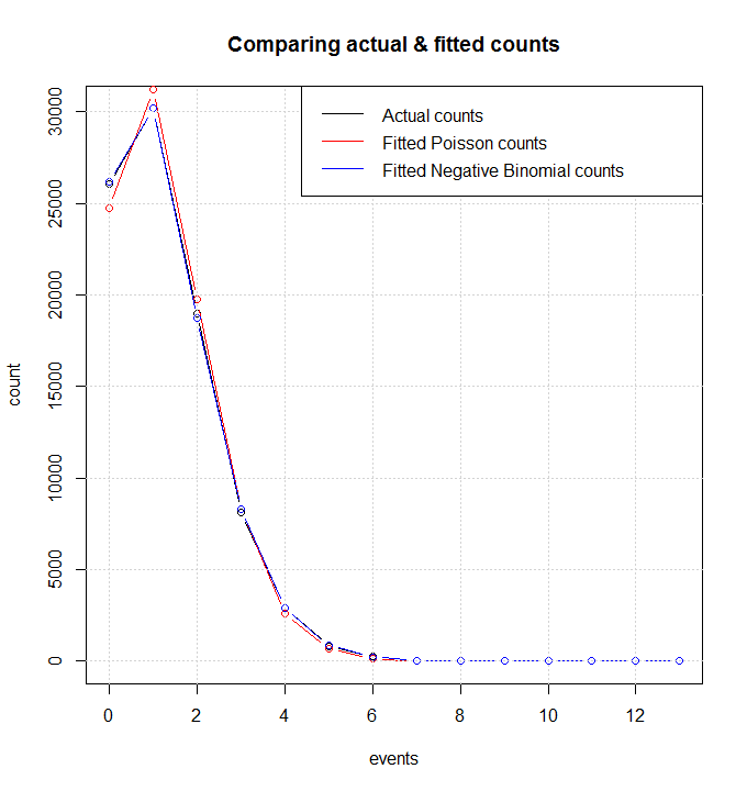
As you rightly suspected, the counts generated by the ML Negative Binomial distribution are closer to your original count data than those of the ML Poisson distribution we have fitted.

This is even more apparent in a chart:

    plot(count ~ events, count.data, 'b', col='black', 
          main='Comparing actual & fitted counts')
    lines(count.data$events, fitted.poisson.counts, 'b', 
            col='red')
    lines(count.data$events, fitted.negbin.counts, 'b', 
         col='blue')
    grid()
    legend("topright", legend=c('Actual counts', 
          'Fitted Poisson counts', 
          'Fitted Negative Binomial counts'), lty=1, 
           col=c('black', 'red', 'blue'))