The limit of "unit-variance" ridge regression estimator when $\lambda\to\infty$

Question

Consider ridge regression with an additional constraint requiring that $\hat{\mathbf y}$ has unit sum of squares (equivalently, unit variance); if needed, one can assume that $\mathbf y$ has unit sum of squares as well:

$$\hat{\boldsymbol\beta}_\lambda^* = \arg\min\Big\{\|\mathbf y - \mathbf X \boldsymbol \beta\|^2+\lambda\|\boldsymbol\beta\|^2\Big\} \:\:\text{s.t.}\:\: \|\mathbf X \boldsymbol\beta\|^2=1.$$

What is the limit of $\hat{\boldsymbol\beta}_\lambda^*$ when $\lambda\to\infty$?

---

Here are some statements that I believe are true:

1. When $\lambda=0$, there is a neat explicit solution: take OLS estimator $\hat{\boldsymbol\beta}_0=(\mathbf X^\top \mathbf X)^{-1}\mathbf X^\top \mathbf y$ and normalize it to satisfy the constraint (one can see this by adding a Lagrange multiplier and differentiating): $$\hat{\boldsymbol\beta}_0^* = \hat{\boldsymbol\beta}_0 \big/ \|\mathbf X\hat{\boldsymbol\beta}_0\|.$$

2. In general, the solution is $$\hat{\boldsymbol\beta}_\lambda^*=\big((1+\mu)\mathbf X^\top \mathbf X + \lambda \mathbf I\big)^{-1}\mathbf X^\top \mathbf y\:\:\text{with $\mu$ needed to satisfy the constraint}.$$I don't see a closed form solution when $\lambda >0$. It seems that the solution is equivalent to the usual RR estimator with some $\lambda^*$ normalized to satisfy the constraint, but I don't see a closed formula for $\lambda^*$.

3. When $\lambda\to \infty$, the usual RR estimator $$\hat{\boldsymbol\beta}_\lambda=(\mathbf X^\top \mathbf X + \lambda \mathbf I)^{-1}\mathbf X^\top \mathbf y$$ obviously converges to zero, but its direction $\hat{\boldsymbol\beta}_\lambda \big/ \|\hat{\boldsymbol\beta}_\lambda\|$ converges to the direction of $\mathbf X^\top \mathbf y$, a.k.a. the first partial least squares (PLS) component.

Statements (2) and (3) together make me think that perhaps $\hat{\boldsymbol\beta}_\lambda^*$ also converges to the appropriately normalized $\mathbf X^\top \mathbf y$, but I am not sure if this is correct and I have not managed to convince myself either way.

Answer 1

#A geometrical interpretation

The estimator described in the question is the Lagrange multiplier equivalent of the following optimization problem:

$$\text{minimize $f(\beta)$ subject to $g(\beta) \leq t$ and $h(\beta) = 1$ } $$

$$\begin{align} f(\beta) &= \lVert y-X\beta \lVert^2 \\ g(\beta) &= \lVert \beta \lVert^2\\ h(\beta) &= \lVert X\beta \lVert^2 \end{align}$$

which can be viewed, geometrically, as finding the smallest ellipsoid $f(\beta)=\text{RSS }$ that touches the intersection of the sphere $g(\beta) = t$ and the ellipsoid $h(\beta)=1$

---

Comparison to the standard ridge regression view

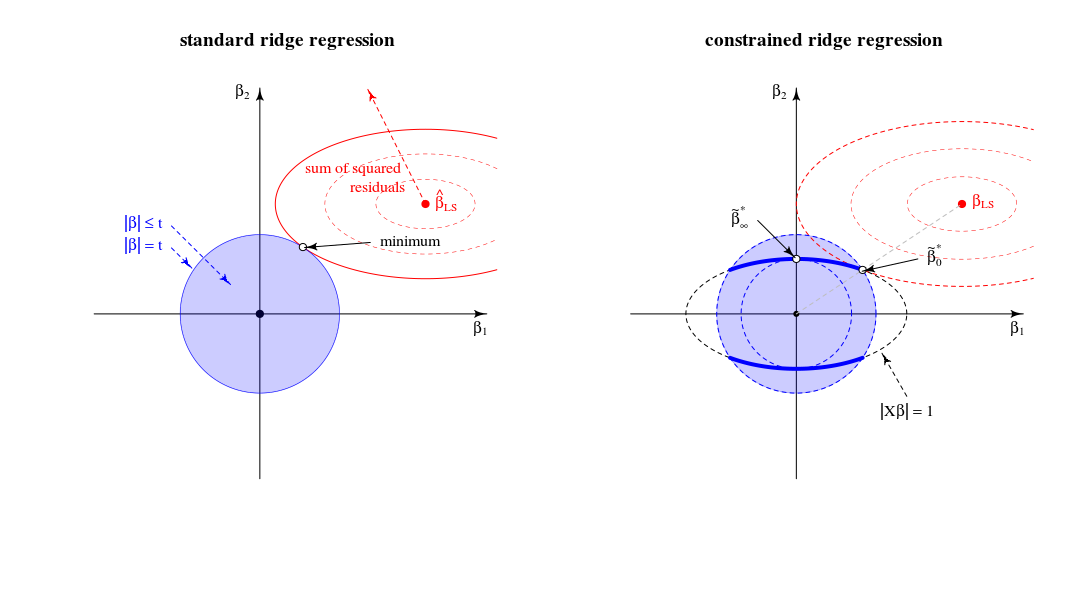
In terms of a geometrical view this changes the old view (for standard ridge regression) of the point where a spheroid (errors) and sphere ($\|\beta\|^2=t$) touch. Into a new view where we look for the point where the spheroid (errors) touches a curve (norm of beta constrained by $\|X\beta\|^2=1$). The one sphere (blue in the left image) changes into a lower dimension figure due to the intersection with the $\|X\beta\|=1$ constraint.

In the two dimensional case this is simple to view.

When we tune the parameter $t$ then we change the relative length of the blue/red spheres or the relative sizes of $f(\beta)$ and $g(\beta)$ (In the theory of Lagrangian multipliers there is probably a neat way to formally and exactly describe that this means that for each $t$ as function of $\lambda$, or reversed, is a monotonous function. But I imagine that you can see intuitively that the sum of squared residuals only increases when we decrease $||\beta||$.)

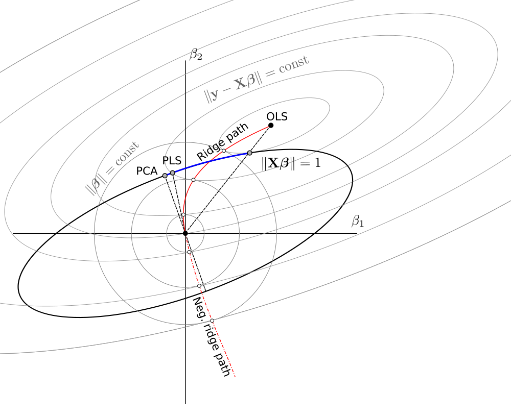
The solution $\beta_\lambda$ for $\lambda=0$ is as you argued on a line between 0 and $\beta_{LS}$

The solution $\beta_\lambda$ for $\lambda \to \infty$ is (indeed as you commented) in the loadings of the first principal component. This is the point where $\lVert \beta \rVert^2$ is the smallest for $\lVert \beta X \rVert^2 = 1$. It is the point where the circle $\lVert \beta \rVert^2=t$ touches the ellipse $|X\beta|=1$ in a single point.

In this 2-d view the edges of the intersection of the sphere $\lVert \beta \rVert^2 =t$ and spheroid $\lVert \beta X \rVert^2 = 1$ are points. In multiple dimensions these will be curves

(I imagined first that these curves would be ellipses but they are more complicated. You could imagine the ellipsoid $\lVert X \beta \rVert^2 = 1$ being intersected by the ball $\lVert \beta \rVert^2 \leq t$ as some sort of ellipsoid frustum but with edges that are not a simple ellipses)

---

##Regarding the limit $\lambda \to \infty$

At first (previous edits) I wrote that there will be some limiting $\lambda_{lim}$ above which all the solutions are the same (and they reside in the point $\beta^*_\infty$). But this is not the case

Consider the optimization as a LARS algorithm or gradient descent. If for any point $\beta$ there is a direction in which we can change the $\beta$ such that the penalty term $|\beta|^2$ increases less than the SSR term $|y-X\beta|^2$ decreases then you are not in a minimum.

• In normal ridge regression you have a zero slope (in all directions) for $|\beta|^2$ in the point $\beta=0$. So for all finite $\lambda$ the solution can not be $\beta = 0$ (since an infinitesimal step can be made to reduce the sum of squared residuals without increasing the penalty).
• For LASSO this is not the same since: the penalty is $\lvert \beta \rvert_1$ (so it is not quadratic with zero slope). Because of that LASSO will have some limiting value $\lambda_{lim}$ above which all the solutions are zero because the penalty term (multiplied by $\lambda$) will increase more than the residual sum of squares decreases.
• For the constrained ridge you get the same as the regular ridge regression. If you change the $\beta$ starting from the $\beta^*_\infty$ then this change will be perpendicular to $\beta$ (the $\beta^*_\infty$ is perpendicular to the surface of the ellipse $|X\beta|=1$) and $\beta$ can be changed by an infinitesimal step without changing the penalty term but decreasing the sum of squared residuals. Thus for any finite $\lambda$ the point $\beta^*_\infty$ can not be the solution.

---

##Further notes regarding the limit $\lambda \to \infty$

The usual ridge regression limit for $\lambda$ to infinity corresponds to a different point in the constrained ridge regression. This 'old' limit corresponds to the point where $\mu$ is equal to -1. Then the derivative of the Lagrange function in the normalized problem

$$2 (1+\mu) X^{T}X \beta + 2 X^T y + 2 \lambda \beta$$ corresponds to a solution for the derivative of the Lagrange function in the standard problem

$$2 X^{T}X \beta^\prime + 2 X^T y + 2 \frac{\lambda}{(1+\mu)} \beta^\prime \qquad \text{with $\beta^\prime = (1+\mu)\beta$}$$

Answer 2

This is an algebraic counterpart to @Martijn's beautiful geometric answer.

First of all, the limit of $$\hat{\boldsymbol\beta}_\lambda^* = \arg\min\Big\{\|\mathbf y - \mathbf X \boldsymbol \beta\|^2+\lambda\|\boldsymbol\beta\|^2\Big\} \:\:\text{s.t.}\:\: \|\mathbf X \boldsymbol\beta\|^2=1$$ when $\lambda\to\infty$ is very simple to obtain: in the limit, the first term in the loss function becomes negligible and can thus be disregarded. The optimization problem becomes $$\lim_{\lambda\to\infty}\hat{\boldsymbol\beta}_\lambda^* = \hat{\boldsymbol\beta}_\infty^* = \operatorname*{arg\,min}_{\|\mathbf X \boldsymbol\beta\|^2=1}\|\boldsymbol\beta\|^2 \sim \operatorname*{arg\,max}_{\| \boldsymbol\beta\|^2=1}\|\mathbf X\boldsymbol\beta\|^2,$$ which is the first principal component of $\mathbf X$ (appropriately scaled). This answers the question.

---

Now let us consider the solution for any value of $\lambda$ that I referred to in point #2 of my question. Adding to the loss function the Lagrange multiplier $\mu(\|\mathbf X\boldsymbol\beta\|^2-1)$ and differentiating, we obtain

$$\hat{\boldsymbol\beta}_\lambda^*=\big((1+\mu)\mathbf X^\top \mathbf X + \lambda \mathbf I\big)^{-1}\mathbf X^\top \mathbf y\:\:\text{with $\mu$ needed to satisfy the constraint}.$$

How does this solution behave when $\lambda$ grows from zero to infinity?

• When $\lambda=0$, we obtain a scaled version of the OLS solution: $$\hat{\boldsymbol\beta}_0^* \sim \hat{\boldsymbol\beta}_0.$$

• For positive but small values of $\lambda$, the solution is a scaled version of some ridge estimator: $$\hat{\boldsymbol\beta}_\lambda^* \sim \hat{\boldsymbol\beta}_{\lambda^*}.$$

• When $\lambda=\|\mathbf X\mathbf X^\top \mathbf y\|$, the value of $(1+\mu)$ needed to satisfy the constraint is $0$. This means that the solution is a scaled version of the first PLS component (meaning that $\lambda^*$ of the corresponding ridge estimator is $\infty$): $$\hat{\boldsymbol\beta}_{\|\mathbf X\mathbf X^\top \mathbf y\|}^* \sim \mathbf X^\top \mathbf y.$$

• When $\lambda$ becomes larger than that, the necessary $(1+\mu)$ term becomes negative. From now on, the solution is a scaled version of a pseudo-ridge estimator with negative regularization parameter (negative ridge). In terms of directions, we are now past ridge regression with infinite lambda.

• When $\lambda\to\infty$, the term $\big((1+\mu)\mathbf X^\top \mathbf X + \lambda \mathbf I\big)^{-1}$ would go to zero (or diverge to infinity) unless $\mu = -\lambda/ s^2_\mathrm{max} + \alpha$ where $s_\mathrm{max}$ is the largest singular value of $\mathbf X=\mathbf{USV}^\top$. This will make $\hat{\boldsymbol\beta}_\lambda^*$ finite and proportionate to the first principal axis $\mathbf V_1$. We need to set $\mu = -\lambda/ s^2_\mathrm{max} + \mathbf U_1^\top \mathbf y -1$ to satisfy the constraint. Thus, we obtain that $$\hat{\boldsymbol\beta}_\infty^* \sim \mathbf V_1.$$

---

Overall, we see that this constrained minimization problem encompasses unit-variance versions of OLS, RR, PLS, and PCA on the following spectrum:

$$\boxed{\text{OLS} \to \text{RR} \to \text{PLS} \to \text{negative RR} \to \text{PCA}}$$

This seems to be equivalent to an obscure (?) chemometrics framework called "continuum regression" (see https://scholar.google.de/scholar?q="continuum+regression", in particular Stone & Brooks 1990, Sundberg 1993, Björkström & Sundberg 1999, etc.) which allows the same unification by maximizing an ad hoc criterion $$\mathcal T = \operatorname{corr}^2(\mathbf y, \mathbf X \boldsymbol\beta)\cdot \operatorname{Var}^\gamma(\mathbf X\boldsymbol\beta) \;\;\text{s.t.}\;\;\|\boldsymbol\beta\|=1.$$ This obviously yields scaled OLS when $\gamma=0$, PLS when $\gamma=1$, PCA when $\gamma\to\infty$, and can be shown to yield scaled RR for $0<\gamma<1$ and scaled negative RR for $1<\gamma<\infty$, see Sundberg 1993.

Despite having quite a bit of experience with RR/PLS/PCA/etc, I have to admit I have never heard about "continuum regression" before. I should also say that I dislike this term.

---

A schematic that I did based on the @Martijn's one:

Update: Figure updated with the negative ridge path, huge thanks to @Martijn for suggesting how it should look. See my answer in Understanding negative ridge regression for more details.