A transformation from uniform random variable to Gaussian mixture

Question

I am attempting to describe a prior_transform for a multivariate Gaussian mixture in order to estimate the evidence integral of that prior convolved with another likelihood distribution. This is nested sampling for integration (not inference at the moment). The "why" is not so important at the moment.

Basically I need a way to transform N independent uniform distributions into a N-dimensional gaussian mixture model (for which I know all the weights, covariances, and means). This is not sampling since my samples are already drawn for me from uniform distributions.

I have a method for transforming to a single multivariate gaussian (using Cholesky Transformation) but I'm not sure how to "upgrade" that to a mixture.

The method I have at the moment is basically the same as in here

1. Get N+1 independent uniform distributions (N dimensions + 1 identifier)
2. Partition the range of [0, 1] based on the weights of the mixture model.
3. Map those partitions to each gaussian in the mixture model.
4. Choose the relevant gaussian from the first uniform distribution using the partitions.
5. Transform the remaining N uniform distributions into the relevant multivariate Gaussian chosen by the partitioned using Cholesky transformation

This will generate the mixture that I want but partitioning a uniform distribution feels like the wrong thing to do when using a prior_transform which takes continuous uniformly distributed random variables.

Is this method appropriate for nested sampling integration?

Is there a better way (continuous mapping) than this method here? (Some form of averaging technique maybe?)

Many thanks

Answer 1

Your approach is correct and good, especially if the components are distant from each other.

An alternative could be to go one coordinate at a time and think about the conditional probability distribution.

Specifically, the CDF of the first parameter is just the weighted sum of the CDFs of the components. Now that you have picked and sampled the first parameter $x_1$ in the transform, you can look at the second parameter. Think about the conditional $P(x_2|x_1)$. It will again be a mixture of gaussians, namely evaluating the components at $x_1$. And so on.

This is mentioned here: https://johannesbuchner.github.io/UltraNest/priors.html#Dependent-priors

Answer 2

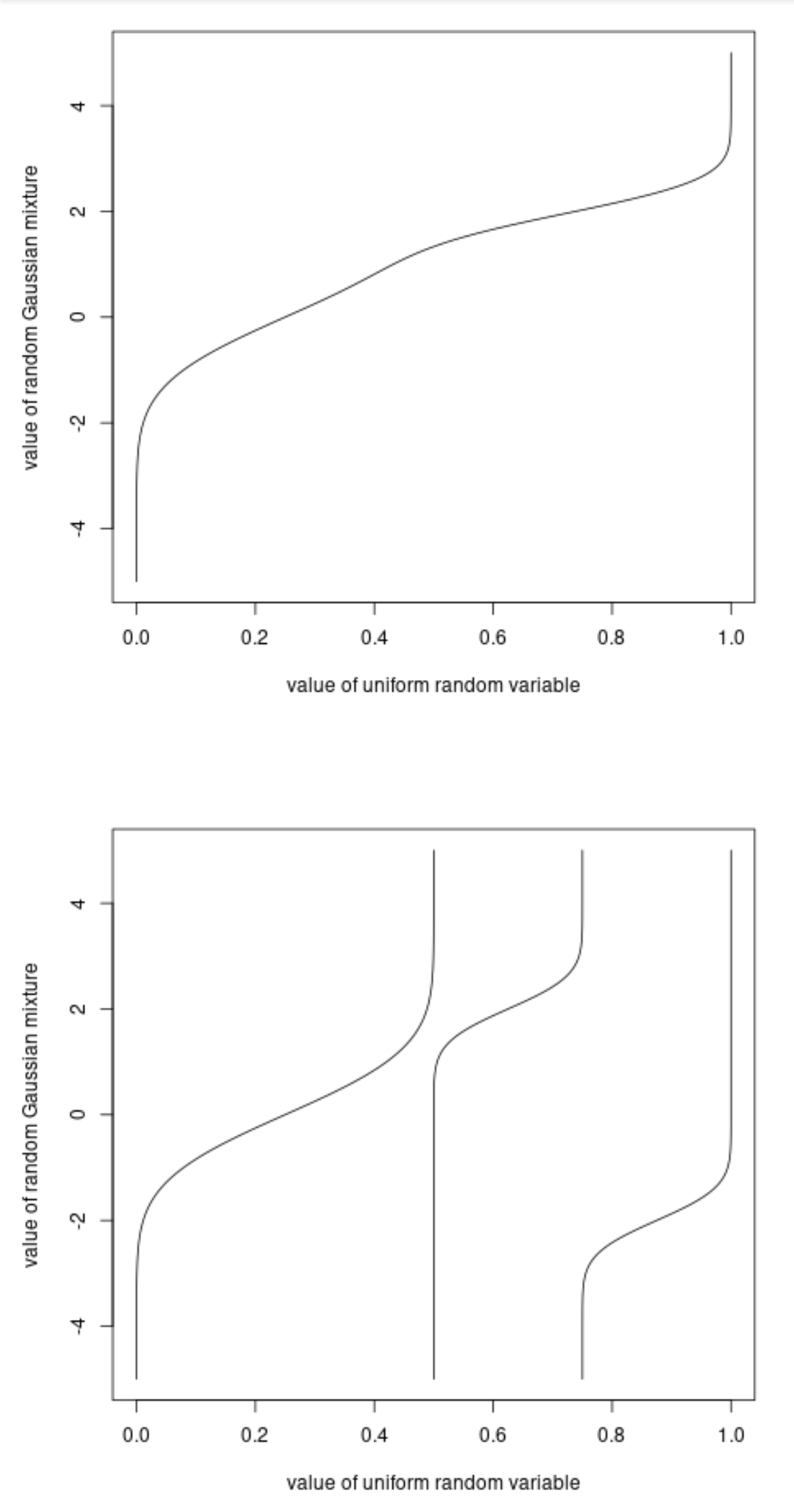
Example with a Gaussian mixture of $$50\%\quad \mathcal{N}(\mu = 0,\sigma = 1) + 25\%\quad \mathcal{N}(\mu = -2,\sigma = 0.5) + 25\%\quad \mathcal{N}(\mu = 2,\sigma = 0.5)$$

You want to sample variables from this Gaussian mixture using inverse transform sampling.

You can do this via a map that is the quantile function in the upper image.

But just as well you can split that map up, like you do, and use 3 seperate quantile functions.