Do these standardized residuals show heteroskedasticity?

Question

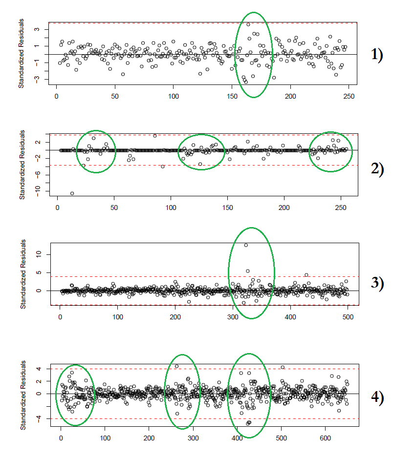
I'm practising in the individuation of heteroskedasticity from the standardized residuals.

I know that, if the time series is homoskedastic, the spread of the residuals should be constant and random around zero-mean.

About my problem, I'm having trouble in the interpretation of the followings plots. I evidenced (with the colour green) the significant parts that, in my opinion, could suggest me that the time series has heteroskedasticity.

The parts that I pointed out, are significant or they are just anomalies? Any help would be appreciated

---

Edit

I add the text from the exercise where I found the standardized residuals of graph 2.

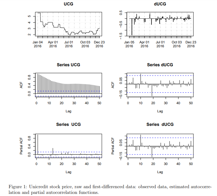
The time series of interest is the Unicredit stock price index at Milan stock market, from 2015-01-02 to 2016-12-23. Figure 1 shows the raw (UCG) and first differenced (dUCG) data together with the estimated autocorrelation and partial autocorrelation functions. The following ARIMA(0, 1, 1) model has been fitted:

Call:
arima(x = UCG, order = c(0, 1, 1))

Coefficients:
          ma1
       0.0253
s.e.   0.0620

sigma^2 estimated as 0.01808: log likelihood = 149.24, aic = -296.47

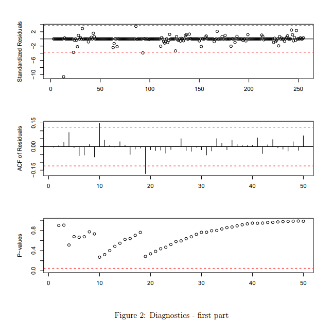
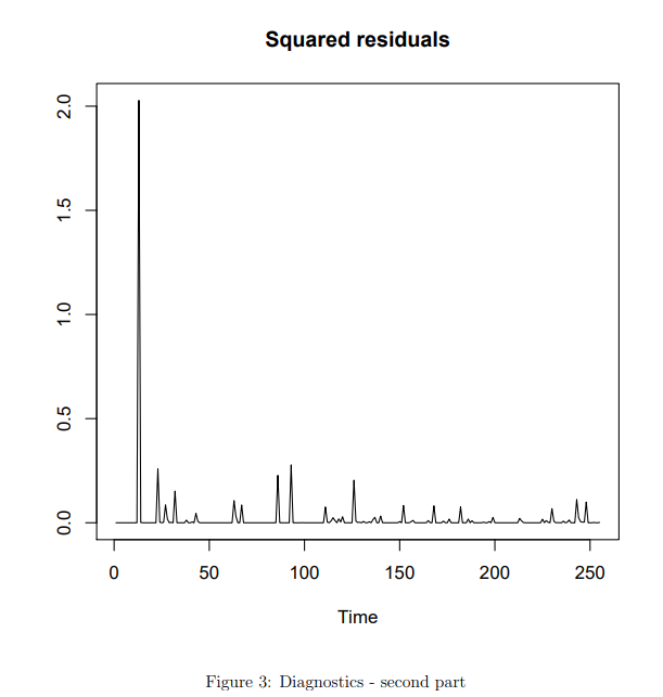
The diagnostics on the residuals are shown in Figure 2 and 3

As you can see the exercise doesn't give me a QQnormal plot in order to identify the distribution of my residuals (in this case the residuals of graph 2, first picture).

Is there another way to confirm if the standardized residuals show homoskedasticity or not?

Answer 1

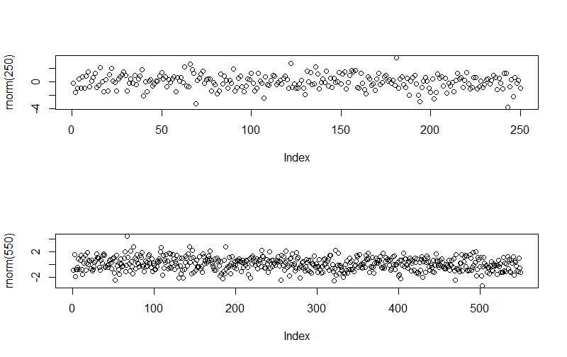
Experienced practitioners know the usual aspect of every graph and are able to tell whether (and how) a given graph deviates from the usual case. Since I'm not an experienced practitioner, I need to generate benchmark graphics to compare with my problem graphics. This way it's easier to tell if the situation depicted in a given graph is different from the expected situation I have simulated.

Faced with your problem, I would try to simulate a graph of residuals from an homoskedastic population and compare it with your graphs. The problem now is that we need to know what distribution are we going to sample from. Any insight on what distribution residuals are expected to follow in your problem would be very useful. However, since I don't have such insight, I would start trying with a normal distribution:

par(mfrow=c(2,1))
plot(rnorm(250))
plot(rnorm(550))

Just by comparing with those graphs I would say:

• Some outliers can be expected even in an homoskedastic distribution.
• Your outliers are a lot more far away than mine. If your residuals are supposed to be normally distributed, that could be a symptom of heteroskedacity. However, it could also be just a symptom that residuals follow a distribution with heavy tails.

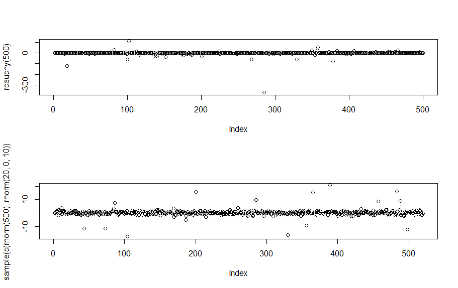
Let's try what happens with a couple of heavy-tailed distributions:

plot(rcauchy(500))
plot(sample(c(rnorm(500),rnorm(20,0,10))))

Those look a lot more similar to your graphs - in fact, there are a few places where we could add green ellipses like yours.

Therefore, although formal tests allow to diagnose more accurately (as Michael Grogan points in his answer), I would say that your residuals don't look like coming from a Gaussian distribution with uniform variance. If they are supposed to be Gaussian, they may be heteroskedastic (or have another problem). If they aren't supposed to be Gaussian, they may just be following a heavy-tailed distribution with uniform variance.

Addition after edit in question:

In the UCG series I see a many periods of several days or weeks with no visible change with days of dramatic changes between days. This leads to a dUCG series with a lot of zero (or maybe near zero) values. With such data most models are likely to get good fits in the quiet periods and large residuals for the fast moving days. Therefore, residuals are likely to follow a heavy tailed distribution and I wouldn't attribute to heteroskedacity the outliers you marked with green ellipses.

Answer 2

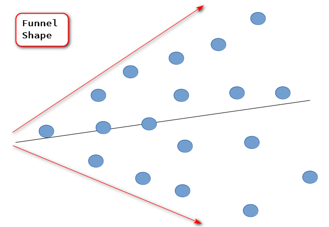
The most common visual clue to heteroscedasticity is a "funnel-shape", where we can clearly see an uneven distribution of variance across our residuals:

This does not particularly appear to be the case with your data, and you might find that the data is homoscedastic even with some anomalies as is this case with your data.

However, the only clinical way to diagnose the presence of heteroscedasticity is through a formal test, such as Breusch-Pagan.

I take it you are using R, so the test can be run using bptest, through use of the lmtest library.

Suppose there is a regression called reg1. Here's some sample output:

> reg1<-lm(y ~ x1 + x2 + x3, data=mydata)
> library(lmtest)
> bptest(reg1)

studentized Breusch-Pagan test

data:  reg1
BP = 3.8512, df = 3, p-value = 0.278

In your case, I would run a formal test as above first to diagnose more accurately. Graphs can provide a visual clue, but they are not the be all and end all.