Controlling variables in causal diagrams

Question

I'm reading "The book of why" by Judea Pearl and although I understand qualitatively what he is saying when it comes to the bias introduced by controlling for an incorrect variable (a collider, for instance), I can't visualise the flow of association/correlation that results from such control.

What happens to the diagram below when I control for B (colored in white)? Why is there a biasing path if I control for B but not if control for C?

Why does controlling for B in the diagram here introduce bias?

Answer 1

This is more of a comment, in response to comments to Ed Rigdon's answer:

I understand that I shouldn’t control for B because it’s a collider. I want to know how the diagram looks when a variable is controlled for. Then I would be able to see everything explicitly

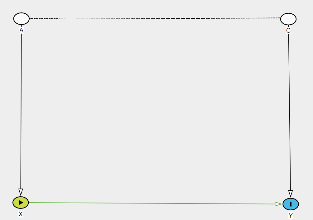
A good way to do this is by drawing the conditional graph by a process called graphical moralization. The steps are very simple (this is quoted almost verbatim from Greenland and Pearl, 2017) where I have just changed the variable names to match the ones in the question:

1. If B is a collider, join (marry) all pairs of parents of B by undirected arcs (here, a dashed line will be used).
2. Similarly, if A is an ancestor of B and a collider, join all pairs of parents of A by undirected arcs. [obviously this is not the case here]
3. Erase B and all arcs connecting B to other variables.

So we arrive at the following graph:

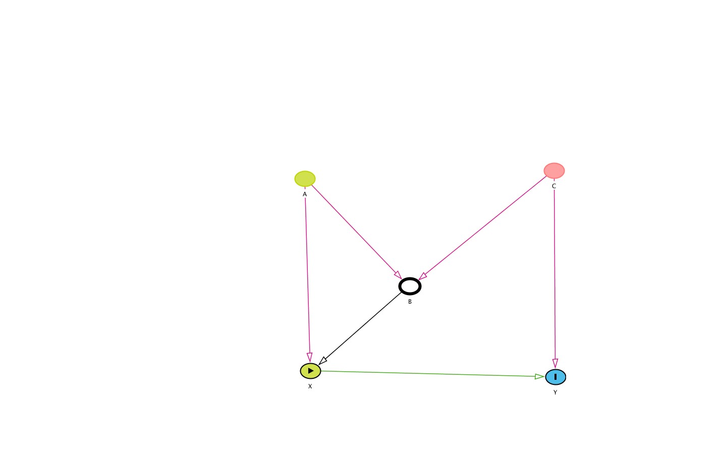
Note that this is not a DAG because of the presence of the dashed line. To continue using DAG theory we must retain B and use the reasoning in Noah's answer where the backdoor path is shown as $X \leftarrow A \rightarrow \fbox B \leftarrow C \rightarrow Y$

Finally I often find it instructive to do simple simulation so here I simulate data according to the original DAG and show what happens when controlling for the collider:

> set.seed(15)
> N <- 100
> A <- rnorm(N, 10, 2)
> C <- rnorm(N, 5, 1)
> B <- A + C + rnorm(N)
> X <- A + B + rnorm(N)
> Y <- X + C + rnorm(N)

> m0 <- lm(Y ~ X)
> summary(m0)

Coefficients:
            Estimate Std. Error t value Pr(>|t|)    
(Intercept)  3.28681    0.87685   3.748 0.000301 ***
X            1.06439    0.03411  31.203  < 2e-16 ***

So we obtain good estimates for the effect of X. However:

> m1 <- lm(Y ~ X + B)
> summary(m1)

Coefficients:
            Estimate Std. Error t value Pr(>|t|)    
(Intercept)  2.82040    0.82263   3.429 0.000892 ***
X            0.68665    0.09811   6.999 3.36e-10 ***
B            0.66931    0.16452   4.068 9.65e-05 ***

Now we have a biased estimate for X

Answer 2

In the model, B = A + C, and A and C are orthogonal. If you hold B constant, you induce covariance between A and C. Say you hold B constant at 10. Then, if A is 7, C is 3. If A is 6, then C is 4. This creates a confound for the X -> Y relationship, a backdoor path from X through A through the covariance with C to Y.

C is a confound for the X -> Y relationship because X and Y are joint descendants of C. Controlling for C negates that joint dependence. You don't need to control for B because B by itself is not a confound--Y is not a descendant of B, except through X.

One of the tough parts of interpreting diagrams is looking for the paths that are not there. Those omissions can be the most important part of the diagram, but without practice they will not be the focus of our attention.

Answer 3

There are seven rules of association. In the first four, $R$ and $T$ are associated with each other:

$$R \rightarrow T$$ $$R \rightarrow S \rightarrow T$$ $$R \leftarrow S \rightarrow T$$ $$R \rightarrow \fbox S \leftarrow T$$

In the second three, $R$ and $T$ are not associated with each other through the path:

$$R \rightarrow \fbox S \rightarrow T$$ $$R \leftarrow \fbox S \rightarrow T$$ $$R \rightarrow S \leftarrow T$$

A box around a variable means we are conditioning on the variable.

The path $X \leftarrow A \rightarrow B \leftarrow C \rightarrow Y$, when not conditioning on $B$, is a closed path, meaning that $X$ and $Y$ are not associated with each other through this path. This is because the chain of association breaks when two arrows point to the same variable in a path (here, two arrows point to $B$). In this case, $B$ is called a collider.

Conditioning on $B$ opens the path of association. That is, $X \leftarrow A \rightarrow \fbox B \leftarrow C \rightarrow Y$ leaves open the association between $X$ and $Y$ because conditioning on a collider or a descendant of a collider opens the path of association. Other paths between $X$ and $Y$ may be open or closed, but when through this particular pathway, they are associated. This association is "noncausal" because it's an association that does not represent the causal effect of $X$ on $Y$.