A natural (and perhaps naive) way to model mortality would be a binomial model, i.e.,
$$
x \sim \text{Binomial}(n, p)
$$
Here $x$ is the number of deaths, $n$ is the total number of people infected, and $p$ is the mortality rate, or the probability of dying given that you have the disease.
When we say something is distributed according to a binomial distribution, we mean that the observed counts $x$ are the result of $n$ independent trials, each with probability of "success" (in this case, death) $p$. These are usually termed "Bernoulli trials".
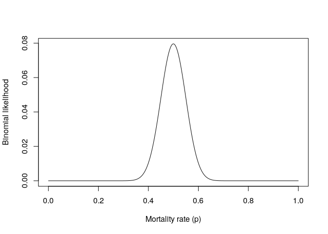
We can now examine the likelihood of $p$ given $x$ and $n$ -- i.e., how likely it would be to see the data we have observed, given different values of $p$. Imagine we had 100 cases, 50 of which resulted in deaths:
n <- 100
x <- 50
s <- seq(0, 1, length.out=1000)
plot(
  s, dbinom(x, size = n, prob = s), type="l",
  xlab = "Mortality rate (p)", ylab = "Binomial likelihood"
)

This shows that a point estimate (the maximum likelihood estimate) would be 0.5, which of course makes sense. Something important to consider here is the amount of data we have observed. Since we have a good amount of observations, the likelihood is fairly narrow. This means that there is a relatively small range of values for $p$ for which the data we observed would be likely to occur.
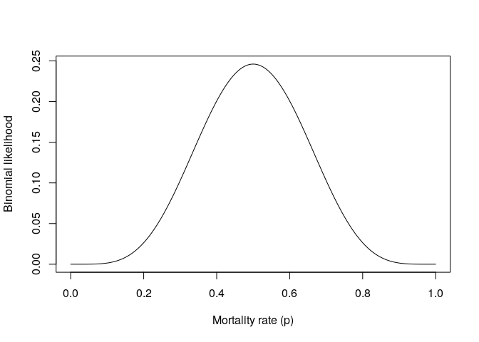
Now, imagine if we had only 10 cases, 5 of which resulted in deaths:
x <- 5
n <- 10
s <- seq(0, 1, length.out=1000)
plot(
  s, dbinom(x, size = n, prob = s), type="l",
  xlab = "Mortality rate (p)", ylab = "Binomial likelihood"
)

When we don't have much information, the likelihood is quite broad, indicating that the data would be fairly likely for a wide range of values for $p$.
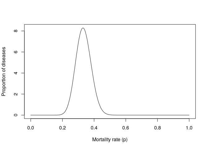
It can be helpful in cases like this to incorporate a prior, or how likely we think different parameter values are, based on our existing knowledge. For example, imagine that we knew that the distribution of mortality rates across all known human diseases looked something like this:
s <- seq(0, 1, length.out=1000)
plot(
  s, dbeta(s, 32, 64), type="l",
  xlab = "Mortality rate (p)", ylab = "Proportion of diseases"
)

This is a Beta prior with $\alpha=32$ and $\beta=64$, i.e.,
$ p \sim \text{Beta}(32, 64)$.
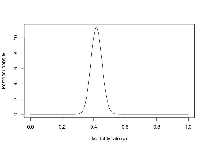
We might want to use this prior information to guide our inferences about the mortality rate of a new disease for which we have very little information. We can combine this prior information with the likelihoods we've already plotted. If you want details about how this is done, one great starting point is this blog by David Robinson. Basically, the posterior distribution over our parameters is a Beta distribution. For parameters we take the $\alpha$ of our prior and add $x$, and take the $\beta$ of our prior and add $n-x$.
s <- seq(0, 1, length.out=1000)
n <- 100
x <- 50
plot(
  s, dbeta(s, shape1 = 32 + x, shape2 = 64 + n - x),
  type="l", xlab = "Mortality rate (p)", ylab = "Posterior density"
)

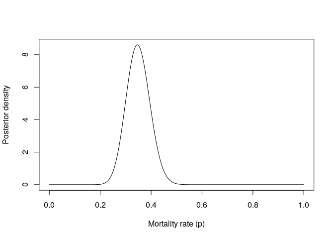
As you can see, this prior information "pulls" our estimates downwards towards the distribution of existing mortality rates. However, if we had strong enough evidence (for example, thousands of infections and deaths) we could still produce an estimate outside of where the prior distribution is concentrated. When we have a small amount of data, a prior can be particularly helpful to avoid results that are purely the result of sampling noise - for example, imagine the first 10 people with a disease happen to die, and the next 90 survive. The estimate after 10 people would be 100%, which is extremely unlikely, given what we've seen about human disease in the past.
s <- seq(0, 1, length.out=1000)
n <- 10
x <- 5
plot(
  s, dbeta(s, shape1 = 32 + x, shape2 = 64 + n - x),
  type="l", xlab = "Mortality rate (p)", ylab = "Posterior density"
)

When we have very little data, this prior information really shrinks our estimates towards what we believe is a reasonable estimate of mortality, given what we've observed in the past about other diseases.
You can continually update this posterior distribution as new data comes in by adding deaths to the $\alpha$ parameter and survivals to the $\beta$ parameter of the Beta distribution.
This is all just general; I have no real expertise in disease modelling. None of the parameters values I've chosen have any basis in reality.

