Limiting distribution of maximum of i.i.d. Gaussians with decreasing variance

Question

Consider a random vector $X^{(m)} = (X^{(m)}_1,\dots,X^{(m)}_m)$ where, for fixed $m$, the elements of $X^{(m)}$ are i.i.d. $\mathcal{N}(0,\sigma^2 / m)$. Define $$Z_m =\max_{k=1,\dots,m}X^{(m)}_k.$$ What can we say about the distribution of $Z_m$ as $m$ gets large? Ideally I'd like a result such of the form $Z_m=\mathcal{O}_p(f(Z))$. Note that this problem is different than the standard problem where the variance is fixed, as is discussed here and here.

Answer 1

The lesson of extreme value theory is that when you rescale the maximum of $m$ iid standard Normal variables by an amount proportional to $\sqrt{2\log m}$ and shift that to a location near $\sqrt{2\log m},$ it converges to the standard Gumbel distribution as $m$ increases.

If first you rescale your $m$ iid Normal variables by $\sqrt{m},$ they become standard Normal, and the preceding applies.

Consequently, for suitable constants $\alpha$ and $\beta,$ $$Z_m \beta \sqrt{2m\log m} - \alpha \sqrt{2\log m}$$ converges to a Gumbel distribution.

In particular, this means we may approximate $Z_m$ closely (in distribution) by

$$Z_m \approx \frac{Y }{\beta \sqrt{2m\log m}} + \frac{\alpha}{\beta\sqrt{m}}$$

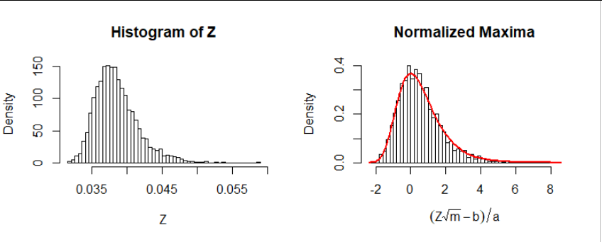
for a Gumbel variate $Y.$ Since the denominators diverge, the (unnormalized) limiting distribution of $Z_m$ is $0$ (in probability). Notice that it does so by being squeezed narrowly around a positive value $\alpha / (\beta\sqrt{m})$ while this central value creeps slowly down towards zero. Here's a histogram with $m=10000$ based on $4000$ such samples:

The red curve plots the limiting Gumbel density, $f(y) = \exp(-e^{-y} - y).$