Having a hard time with the law of the iterated logarithm

Question

Let's say you have infinitely many i.i.d. Bernouilli variables $X_1, X_2, \cdots$ of parameter $p=\frac{1}{2}$. For instance, the binary digits of a random number. Let $S_n = X_1 + \cdots X_n$.

The law of the iterated logarithm (see here) states that $$\lim_{n\rightarrow\infty}\sup \frac{S_n-np}{\sqrt{2np(1-p)\log\log n}}=1.$$

I can't replicate this behavior by simulations no matter what I do. Wikipedia shows a chart explaining why the $\log \log n$ is needed in the formula (see here) but not sure what data it is based on: it goes all the way to $n=\infty$, it can't be real data if it contains an infinite number of observations. In all my tests, the $\log \log n$ makes the $\lim \sup$ tends to 0, not 1.

Now let $$Z_n=\sqrt{n}\cdot\Big(\frac{S_n}{n} - p\Big) = \frac{S_n -np}{\sqrt{n}}.$$

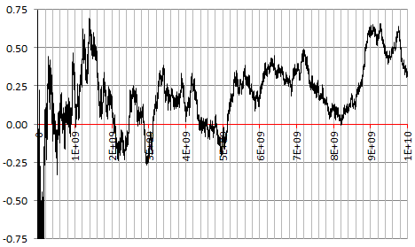
Here $p=\frac{1}{2}$. Of course $Z_n$ is asymptotically normal $N(0,pq)$. So technically $Z_n$ could be arbitrarily high, extremely high, and this happening regularly, suggesting that $\lim \sup Z_n =\infty$. This is in agreement with the law of the iterated logarithm. Yet based on simulations with $n=10^{10}$ and a very good random generator, all evidence suggests that $\lim\sup Z_n$ is bounded by a rather small constant, less than 1. This contradicts the law of the iterated logarithm, it seems.

Below is the chart for $Z_n$ based on 10 billion observations.

It was produced with the following random generator: $Y_{k+1}=3Y_k - \lfloor 3Y_k\rfloor$ with $Y_1=\sqrt{2}$ and $X_k = \lfloor 2Y_k\rfloor \in \{0, 1\}$. This random generator is aperiodic and has other nice features. In this case $p=\frac{1}{2}$.

My question

What am I missing here? Why do my results (and above is one of many tests) seem to contradict the law of the iterated logarithm? Is it the fact that the successive $Z_n$ are highly correlated? But this is assumed too in the law of the iterated algorithm, right? Or am not properly understanding the law of the iterated algorithm or the concept of $\lim \sup$?

Notes about the above random generator

The sequence $Y_n$ is completely wrong after 45 iterations or so due to error (caused by machine precision) propagating exponentially fast from one iteration to the next one. However this is not an issue, it's like starting with a new seed every 40 iterations or so. It is not an issue because the sequence $Y_n$ is ergodic.

Ideally I wanted to use $Y_{k+1}=2Y_k - \lfloor 2Y_k\rfloor$ but in the programming language I used (Perl) the iterates erroneously reached zero after 45 iterations due to the way computations are done by the computer. The computation of $2Y_k$ can be carried very efficiently in base 2, it's just shifting the binary digits.

The speed of computations in the actual version of the generator is significantly improved (by an order of magnitude) if you replace $3Y_k$ by $Y_k + Y_k + Y_k$ in the source code.

Answer 1

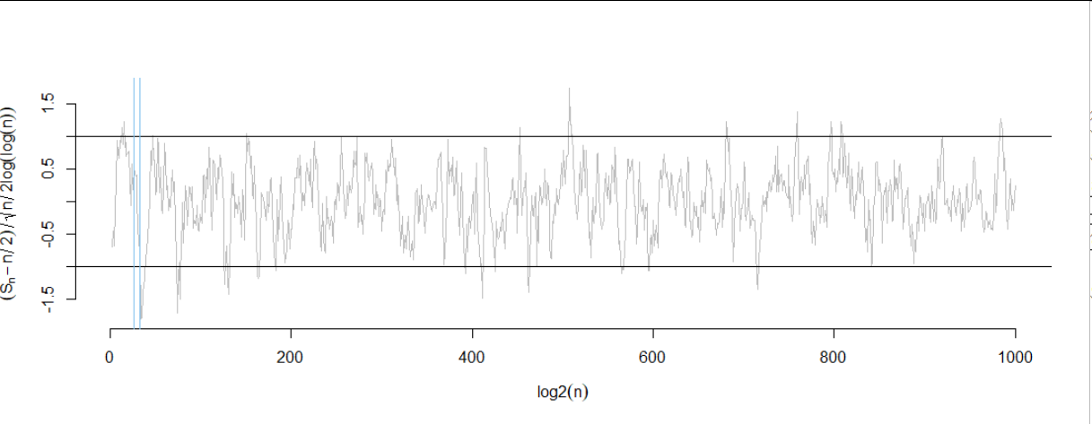
You are looking at a truly tiny simulation. Here's one that went out to $n=2^{1000} \approx 1.07\times 10^{301}:$

(In order to plot it I thinned the walk to $999$ values equally spaced horizontally and connected them with line segments. The actual simulation is, of course, much more detailed than can be shown here :-).)

Clearly this walk repeatedly hits (and slightly exceeds) the $\pm 1$ thresholds. The Law of the Iterated Logarithm says this behavior will continue ad infinitum, with the excursions beyond this threshold growing ever rarer.

The range from $n=10^8$ to $n=10^{10},$ which is basically that visible in your plot, is bounded on the left and right by the light blue lines. In the overall context, we can hardly expect the scaled random walk to vary much within such a narrow interval.

The point is that this law requires you to plot the scaled, standardized random walk on a logarithmic (or even log-log) axis for the index $n.$