Report power if result is statistically significant

Question

We have submitted a paper reporting a statistically significant result. One reviewer asks us to report what is the power to detect a significant association. As there was a previous paper on this issue, we could use the effect size of that paper to do the calculation. However, we are surprised by this comment, and would be happy to know what is your opinion and whether you know of references that discuss calculation of power at posteriori when the result is significant.

---

Thank you very much for your responses.

I should have made clearer that we used a large dataset to run these analyses, so the study is unlikely to be underpowered. However, it involves a complex design, and other than running simulations, there is no simple way to compute power. We are not familiar with simulations to compute power, so I was trying to avoid this :-)

Answer 1

Context: I wrote this answer before the OP clarified that they are working with a large dataset, so the study (probably) has sufficient power. In my post I consider the more common case of a small study with a "significant finding". Imagine, for example, that the article under review presents an estimate of 1.25 in a domain where previous studies about related phonemena have reported estimates in the range [0.9, 1.1]. How does the article's author respond to the reviewer's request for a post-hoc estimate of power to detect an effect of size 1.25?

---

It's hard to argue that it doesn't matter if a study with significant p-value is underpowered. If a study has low power and the null hypothesis is rejected, then the sample statistic is likely to be a biased estimate of the population parameter. Yes, you are lucky to get evidence against the null hypothesis but also likely to be over-optimistic. The reviewer knows this so he asks how much power your study had to detect the effect you detected.

It's not recommended to do post-hoc power estimation. This is a much discussed topic on CV; see references below. In short – if your study was indeed underpowered to detect the true effect size – by doing post-hoc power analysis you compound the issue of overestimating the effect by also overestimating the power. Mathematically, the power at the observed effect is a function of the p-value: if the p-value is small, the post-hoc power is large. It's as if the result is more convincing because the same fact — the null is rejected — gets reported twice.

Okay, so enough bad news. How can you respond to the reviewer? Computing the power retroactively is not meaningful because your study is already done. Instead compute confidence interval(s) for the effect(s) of interest and emphasize estimation, not hypothesis testing. If the power of your study is low, the intervals are wide (as low power means that we can't make precise estimates). If the power of your study is high, the intervals are tight, demonstrating convincingly how much you have learned from your data.

If the reviewer insists on a power calculation, don't compute the power by plugging in the estimated effect for the true effect, aka post-hoc power. Instead do sensitivity power analysis: For example, fix the sample size, the power and the significance level, and determine the range of effect sizes that can be detected. Or fix the sample size and the significance, and plot power as a function of effect size. It will be especially informative to know what the power is for a range of realistic effect sizes.

Daniël Lakens discusses power at great length in Improving Your Statistical Inferences. There is even a section on "What to do if Your Editor Asks for Post-hoc Power?" He has great advice.

References

J. M. Hoenig and D. M. Heisey. The abuse of power. The American Statistician, 55(1):19–24, 2001.
A. Gelman. Don't calculate post-hoc power using observed estimate of effect size. Annals of Surgery, 269(1), 2019.

Do underpowered studies have increased likelihood of false positives?
What is the post-hoc power in my experiment? How to calculate this?
Why is the power of studies that only report significant effects not always 100%?
Post hoc power analysis for a non significant result?

---

This simulation shows that "significant" estimates from underpowered studies are inflated. A study with little power to detect a small effect has more power to detect a large effect. So if the true effect is small and the null hypothesis of no effect is rejected, the estimated effect tends to be larger than the true one.

I simulate 1000 studies with 50%, so about half of the studies have p-value < 0.05. The sample means from those "significant" studies are mostly to the right of the true mean 0.1, ie. they overestimate the true mean, often by a lot.

library("pwr")
library("tidyverse")

# Choose settings for an underpowered study

mu0 <- 0
mu <- 0.1

sigma <- 1
alpha <- 0.05
power <- 0.5

pwr.t.test(d = (mu - mu0) / sigma, power = power, sig.level = alpha, 
           type = "one.sample")
#> 
#>      One-sample t test power calculation 
#> 
#>               n = 386.0261
#>               d = 0.1
#>       sig.level = 0.05
#>           power = 0.5
#>     alternative = two.sided

# Sample size to achieve 50% power to detect mean 0.1 with a one-sided t-test
n <- 387

# Simulate 1,000 studies with low power

set.seed(123)
reps <- 1000

studies <-
  tibble(
    study = rep(seq(reps), each = n),
    x = rnorm(reps * n, mean = mu, sd = sigma)
  )

results <- studies %>%
  group_by(
    study
  ) %>%
  group_modify(
    ~ broom::tidy(t.test(.))
  )

results %>%
  # We are only interested in studies where the null is rejected
  filter(
    p.value < alpha
  ) %>%
  ggplot(
    aes(estimate)
  ) +
  geom_histogram(
    bins = 33
  ) +
  geom_vline(
    xintercept = mu,
    color = "red"
  ) +
  labs(
    x = glue::glue(
        "estimate of true effect {mu} in studies with 
         {100*power}% power"),
    y = "",
    title = "\"Significant\" effect estimates from underpowered 
             studies are inflated"
  )

^{Created on 2022-04-30 by the reprex package (v2.0.1)}

Answer 2

Roughly speaking, observing a significant result in a test with low power means that the observed result is unlikely both under the null hypothesis and under the alternative. So interpreting such a result as evidence in favor of the alternative hypothesis can be problematic.

Now you can say that this is just a wrong interpretation (rejecting the null hypothesis does not mean accepting the alternative), but if there is no evidence in favor of some alternative it's not clear how to interpret the result.

As an extreme example, suppose that someone tries to reject some arbitrary null hypothesis (for example, that there is global warming) by flipping a coin 5 times. If they are lucky enough and observe 5 heads in a row, they can claim that the result is significant ($p < 0.05$) and therefore they reject the null hypothesis. But clearly claiming that global warming doesn't exist based on coin flips is completely meaningless.

The issue here is that such a test has no power (more precisely , the power of the test is equal it's size) - the distribution of the test statistic is exactly the same under both hypotheses.

Notice that in a Bayesian analysis those issues don't exist - in the above case, for example, the posterior probabilities will just be euqal to the prior probabilities of both hypotheses because the test carries no relevant information whatsoever. This is one example of the sometimes problematic aspects of frequentist quantities.

Answer 3

The existing answers provide useful information and arguments, but I disagree with them on what I see as the core question: is it useful to do a post hoc power analysis? I would argue that it IS useful - if you are set on using a Null Hypothesis Statistical Testing framework.

It is absolutely crucial that this analysis is not done with the effect size estimated from the study itself. Instead, I would use either (a) the best estimate based on previous studies that have examined this question, or if this isn't possible, (b) the smallest effect size that would be interesting.

What would such an analysis achieve? It would indicate whether the study was appropriately powered to detect a meaningful effect size. If your study was unlikely to detect the expected effect size, it doesn't mean your finding was wrong - but it is reasonable to be sceptical of the robustness of the analysis and inferences.

Why is it important to not use the effect size estimated in the same study? Because as @dipetkov's answer shows, significant effect sizes are inflated in underpowered studies (and are quite likely to be in the opposite direction of the true effect!). Plugging an inflated estimate into a power calculation would be circular and overestimate the study's power.

That said, I agree with the answers pointing you towards thinking of this in a Bayesian framework. This avoids some of the messiness arising as a result of NHST, which can sometimes struggle for coherence as a result of the "p < 0.05 = truth" fallacy with which it is so tightly enmeshed.

In support of these claims, I'll point you to the same Andrew Gelman letter that @dipetkov's answer does, and also to his blog post about it that makes the same point less formally:

https://statmodeling.stat.columbia.edu/2018/09/24/dont-calculate-post-hoc-power-using-observed-estimate-effect-size/

Gelman, A. (2019). Don’t calculate post-hoc power using observed estimate of effect size. Annals of Surgery, 269(1), e9-e10.

Answer 4

The power of the observed effect is very often equal to a simple one-to-one relationship with the p-value (and the significance level) since both the p-value and the power are dependent on how many standard deviations the effect size is away from zero effect.

As a consequence, such power calculation doesn't add much information.

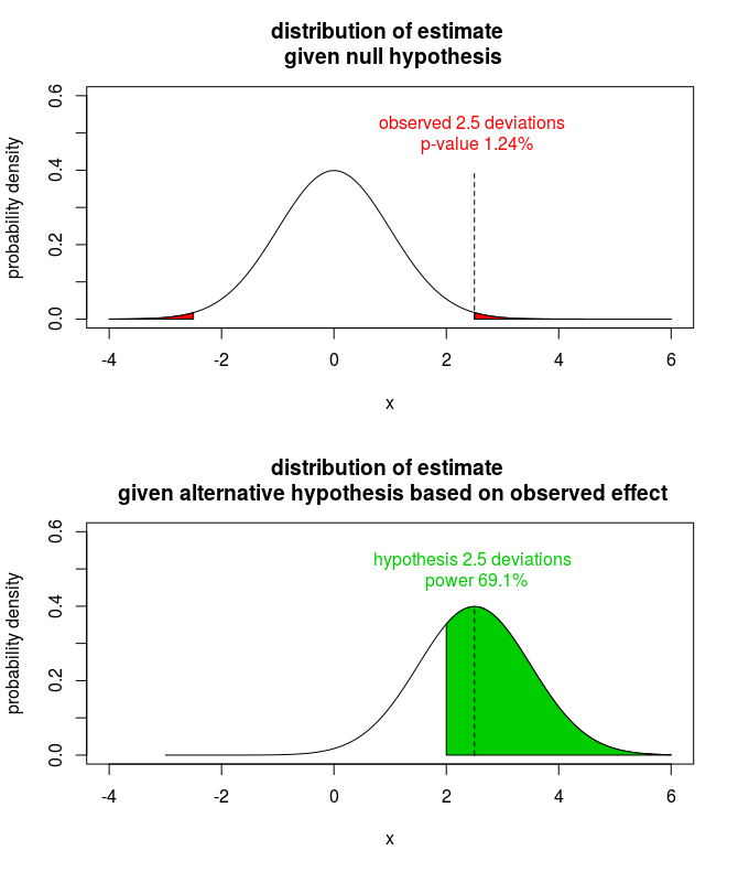
Let's consider this simplistic model in which you have an observation whose likelihood function can be approximated with a normal distribution. Say that the significance level is 5% (or roughly 2 deviations away from zero effect) and we observe an effect with a p-value of 1.24% (or roughly 2.5 deviations away from zero effect) then the power for that observed effect is equal to roughly 69.1% (the probability that the observed effect is more than 2 deviations away from the zero effect given that the true effect is 3 deviations away).

You have a more complex model but often the estimates are approximately equal to a normal distributed variable.

---

More precisely stated. Let some statistic be distributed according to a normal distribution (the simple case of a z-test)

$$T \sim N(\mu,\sigma^2)$$

The p-value for the hypothesis $H_0: \mu = 0$ is a function of the observed statistic $\hat{T}$

$$\text{p-value} = 2\Phi\left( \frac{|\hat{T}|}{\sigma}\right)$$ where $\Phi$ is the cumulative distribution function for a standard normal distribution.

The critical boundary beyond which the absolute value of an observation $\hat{T}$ is considered significant is

$$T_{critical} = \sigma \Phi^{-1}(\alpha/2)$$

The power of the observed effect is the probability to observe a significant result given the alternative $H_a: \mu = \hat{T}$. This is also a function of the observed statistic $\hat{T}$ (along with the significance level $\alpha$ or critical level $T_{critical}$)

$$\text{power} = 1-\Phi\left(\frac{T_{critical}-\hat{T}}{\sigma}\right) + \Phi\left(\frac{-T_{critical}-\hat{T}}{\sigma}\right) $$

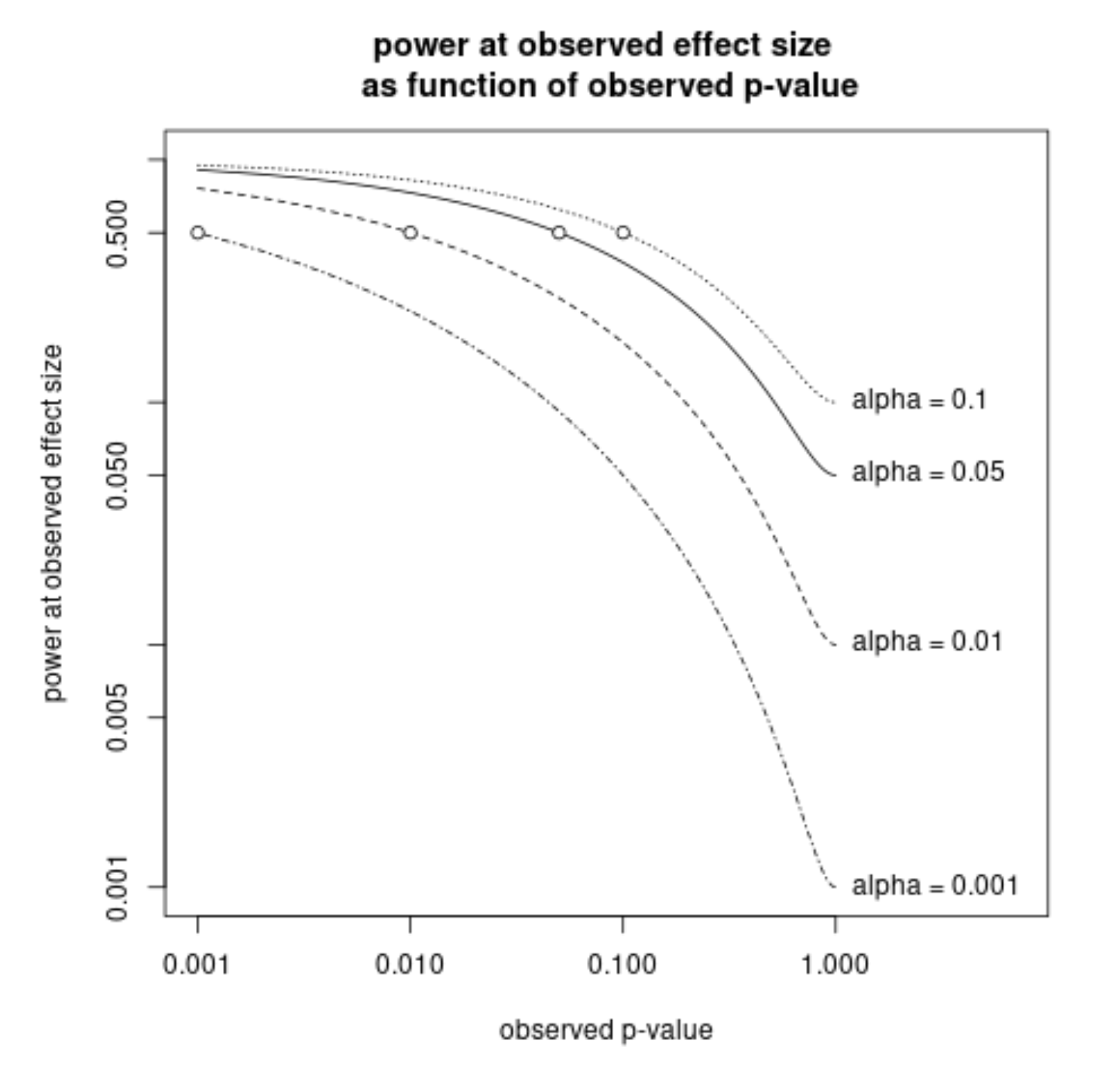
Also added are points where the observed p-value is equal to significance level. The power is close to 50% for an effect size close to the critical effect size of a significance test. If the true effect is close to the critical effect size then (for a symmetric distribution of the sample distribution of the observed effect size) you will more or less observe half the time a smaller effect and half the time a larger effect.

power = function(p,alpha) {
   T_obs = -1*qnorm(p/2)
   T_crit = qnorm(1-alpha/2)
   return(1-pnorm(T_crit-T_obs)+pnorm(-T_crit-T_obs))
}
power = Vectorize(power)


p = seq(0,1,0.001)
plot(p,power(p,0.05), 
     log = "xy", 
     ylab = "power at observed effect size", 
     xlab = "observed p-value", type = "l",
     xlim = c(0.001,7), ylim = c(0.001,1), xaxt = "n")
title("power at observed effect size \n 
       as function of observed p-value", cex=1)
axis(1, at = c(0.001,0.01,0.1,1))

lines(p,power(p,0.01), lty = 2)
lines(p,power(p,0.1), lty = 3)
lines(p,power(p,0.001), lty = 4)

for (p in c(0.001,0.01,0.05,0.1)) {
    text(1,p,paste0("alpha = ",p), pos = 4)
    points(p,power(p,p) , pch = 21, bg = 0)
}

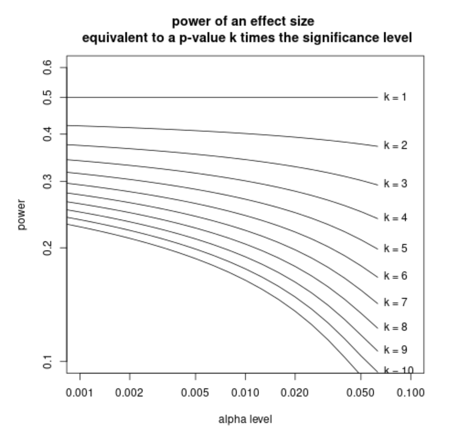
Below is a similar graph considering the power of effect size for which the p-value of an equivalent observation would be $k$ times the significance level.

So if a study reports a p-value ten times above the significance level (fails to reject the null hypothesis), and one wonders what the power would be if the observed effect is the true effect, then this is roughly between 10% to 20% with the higher power for lower significance levels.

a = 10^seq(-5,-1.2,0.1)
plot(a,power(a*11,a),
     type = "l", log = "xy", 
     xlim = c(0.001,0.1), ylim = c(0.1,0.6),
     xlab = "alpha level", ylab="power")
title("power of at an effect size \n 
       equivalent to p-value with k times the significance level", 
      cex = 1)

for (k in 1:10) {
  lines(a,power(a*k,a))
  al = a[length(a)]
  text(al,power(al*k,al), paste0("k = ",k), pos = 4)
}

Answer 5

First, I agree with the answers that say it's a bad idea to do post-hoc power analysis.

Second, most of the answers address the more usual problem that power may be too low. You say (in your edit of your question) that it is a large data set. So, the problem may be that it is overpowered -- that is, able to find that a meaningless relationship is statistically significant.

You could address this issue by a) Giving reasons for not doing post-hoc analysis (see earlier answers) and b) Stressing the effect size and its standard error, rather than the p value. A large sample (other things being equal) allows you to get a precise estimate of parameters.