Understanding percentage of optimal action in Reinforcement Learning

Question

I'm new Reinforcement learning and currently reading Sutton & Barto's book "Reinforcement Learning: An Introduction". In Chapter 2, they compare greedy and non-greedy methods on 10-armed bandit problem. On page 29, the following figure is shown

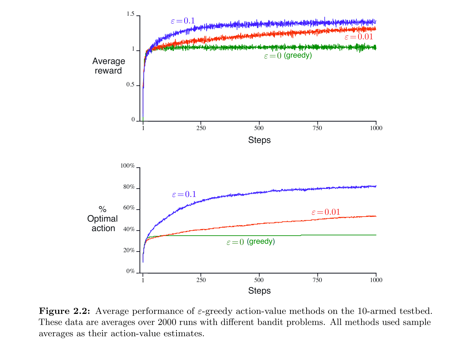
I understand what the upper plot is conveying but I can't wrap my head around on the lower graph. In the text, this is how it is described:

The lower graph shows that the greedy method found the optimal action in only approximately one-third of the tasks. In the other two-thirds, its initial samples of the optimal action were disappointing, and it never returned to it. The $\epsilon$-greedy methods eventually performed better because they continued to explore and to improve their chances of recognizing the optimal action. The $\epsilon$ = 0.1 method explored more, and usually found the optimal action earlier, but it never selected that action more than 91% of the time. The $\epsilon$ = 0.01 method improved more slowly, but eventually would perform better than the $\epsilon$ = 0.1 method on both performance measures shown in the figure.

The questions I have are:

1. For the greedy case, it says "In the other two-thirds, its initial samples of the optimal action were disappointing, and it never returned to it". What do it the text mean by "it never returned to it" and how is that obvious from the plot?

2. How is the case where $\epsilon = 0.01$ outperforming $\epsilon = 0.1$?

In general, I'm confused about what's being measured and the explanation of the results.

Answer 1

1. When a greedy agent first encounters a positive reward after pulling a lever, it sticks to that lever. Levers represent the actions.

   In one-third of the 2000 runs the greedy agent chose an optimal action and stuck with it permanently, because the agent initially sampled higher rewards compared to other actions (which is good). In the remaining runs, the agent probably also chose an optimal action. However, this action resulted in disappointing reward samples (e.g., -1) which was worse than the rewards from the non-optimal actions, so the agent never returned to it (to the optimal action).

   A reward of an action can be far worse than the expected mean in the long run, because the rewards for each arm of the bandit are given according to a random distribution.

   The agent did not return to the optimal action, but how is that obvious from the plot? Not directly, I would say. If we look at the asymptote of the green greedy line in the bottom diagram, we see that it has an intercept of roughly one third. This only means that the agent chooses only in one third of the cases the right action. Our reflection above explains the potential reason.

2. In the first diagram, the red line with ϵ = 0.01 increases faster per step compared to the blue line with ϵ = 0.1. Consequently, the cumulative reward (the integral of the average reward plot) will eventually surpass that of the blue line, possibly around 3000.

   In the second plot, ϵ = 0.01 must eventually outperform ϵ = 0.1, because of the following: The ϵ = 0.01 selects the optimal action in at least 99 out of 100 attempts in average. In the remaining attempt the agent does an exploration, which chooses randomly from all actions. In this case the agent will still pick an optimal action in one out of 10 attempts in average, because there are 10 actions to select from. So the ϵ = 0.01 agent will choose the optimal action in 99% + 1% * 0.1 = 99.1% of the cases if the agent tries and learns long enough. The optimal action ratio for ϵ = 0.1 is similar: 90% + 10% * 0.1 = 91%.