3
$\begingroup$

EDIT: SOLUTION FOUND, SEE BELOW QUESTION

I'm an undergrad writing a very simple lab report in which I'm analysing some data on observed numbers of birds at two different study sites. The exact data frame I'm using was imported off an Excel spreadsheet but I'll replicate the data frame here.

Location <- c(rep("Leighton Moss",6),rep("Eaves Wood",6)
Period<-c(rep(c(rep("Midday",3),rep("Afternoon",3)),2))
Activity<-c(rep(c("Resting","Foraging","Travelling"),4))
Count<-c(88,68,54,30,41,33,13,28,13,55,47,46)

df<-data.frame(Location,Period,Activity,Count)

I want to know if there's an equivalent of Chi-squared test of association for three categorical variables (in this case Location, Period and Activity) as opposed to two.

I ideally want to avoid just doing separate three separate Chi-squared tests for Location vs Activity, Period vs Activity and Location vs Period, but I've found the solution to code for that in case I do need to do that.

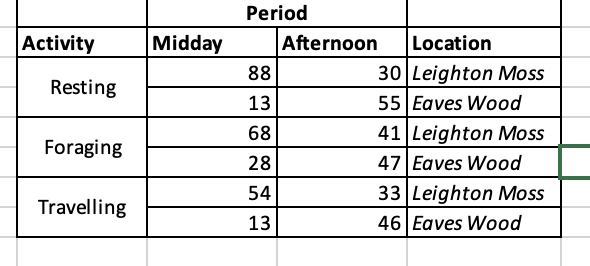
I think I can build a three-way contingency table like this to help:

enter image description here

Beyond that I'm not sure what analysis to do as I think multilinear regression involves a continuous variable? Any code/function that I can use to do this would be great.

Any help y'all can offer is always much appreciated.

Solution

The answer posted below by a fellow commenter had Activity as a covariate which wasn't what I was after; however, I adapted that answer to suit my needs. In the end, I went for a two-pronged analysis.

Firstly, a multinomial logistic regression analysis using the multinom function of the AER package, with Activity as the outcome variable and Period and Location as predictor variables. To do this I listed each observation individually rather than using count data, and the following line of code.

multi_mo<-multinom(Activity ~ Location + Period + Location*Period, data=[data frame name], model=TRUE)

summary(multi_mo)

Secondly, I separated the count data by Activity category, and conducted Poisson regressions on each individual Activity category with Period and Location as covariates. This was just done using the glm function, as shown below.

Resting_Model <- glm(Resting_Count ~ Location + Period + Location:Period,
    family="poisson",
    offset=log(Total_Observations),
    data=[data frame name])

summary(Resting_Model)

Hopefully this helps someone with the same question!

$\endgroup$
3
  • 2
    $\begingroup$ It seems like location and period are your predictor variables, and at each combination of location and period you counted the number of birds engaging in different activities. Is this correct? So in that case maybe the appropriate model would be a multinomial where you are testing the effect of location, period, and their interaction on the probability of an individual bird engaging in each of the 3 activities. Chi-squared test is not really what you want. $\endgroup$
    – qdread
    Commented Apr 20, 2023 at 19:02
  • $\begingroup$ @qdread Yes that's exactly what I'm after! I'll post it over on Stack Exchange, thanks for your help! $\endgroup$ Commented Apr 20, 2023 at 20:09
  • 1
    $\begingroup$ Consider Poisson regression. In a way it is a chi-squared test because the difference in deviance will be distributed as chi-squared. $\endgroup$
    – DWin
    Commented Apr 20, 2023 at 23:45

1 Answer 1

1
$\begingroup$

Here's some code from an effort to clean up some of your R syntax and show a model-comparison approach to using Poisson regression to address your count data problem:

 df<-data.frame( Location = c(rep("Leighton Moss",6),rep("Eaves Wood",6)),
 Period = rep(c(rep("Midday",3),rep("Afternoon",3)),2),
 Activity = rep(c("Resting","Foraging","Travelling"),4),
 Count = c(88,68,54,30,41,33,13,28,13,55,47,46))
 df
#----------------------------
        Location    Period   Activity Count
1  Leighton Moss    Midday    Resting    88
2  Leighton Moss    Midday   Foraging    68
3  Leighton Moss    Midday Travelling    54
4  Leighton Moss Afternoon    Resting    30
5  Leighton Moss Afternoon   Foraging    41
6  Leighton Moss Afternoon Travelling    33
7     Eaves Wood    Midday    Resting    13
8     Eaves Wood    Midday   Foraging    28
9     Eaves Wood    Midday Travelling    13
10    Eaves Wood Afternoon    Resting    55
11    Eaves Wood Afternoon   Foraging    47
12    Eaves Wood Afternoon Travelling    46
#--------------------------------
 glm(Count ~ Location+Period+Activity, data=df, fam="poisson")
#------------------------------
Call:  glm(formula = Count ~ Location + Period + Activity, family = "poisson", 
    data = df)

Coefficients:
          (Intercept)  LocationLeighton Moss           PeriodMidday        ActivityResting     ActivityTravelling  
              3.56042                0.44113                0.04652                0.01081               -0.23133  

Degrees of Freedom: 11 Total (i.e. Null);  7 Residual
Null Deviance:      125.4 
Residual Deviance: 94.55    AIC: 170.1

> mod1 <- glm(Count ~ Location+Period+Activity, data=df, fam="poisson")
> summary(mod1)

Call:
glm(formula = Count ~ Location + Period + Activity, family = "poisson", 
    data = df)

Deviance Residuals: 
    Min       1Q   Median       3Q      Max  
-4.5972  -2.2970  -0.1465   2.1749   3.6698  

Coefficients:
                      Estimate Std. Error z value             Pr(>|z|)    
(Intercept)            3.56042    0.10236  34.783 < 0.0000000000000002 ***
LocationLeighton Moss  0.44113    0.09020   4.891             0.000001 ***
PeriodMidday           0.04652    0.08807   0.528               0.5973    
ActivityResting        0.01081    0.10398   0.104               0.9172    
ActivityTravelling    -0.23133    0.11083  -2.087               0.0369 *  
---
Signif. codes:  0 ‘***’ 0.001 ‘**’ 0.01 ‘*’ 0.05 ‘.’ 0.1 ‘ ’ 1

(Dispersion parameter for poisson family taken to be 1)

    Null deviance: 125.41  on 11  degrees of freedom
Residual deviance:  94.55  on  7  degrees of freedom
AIC: 170.11

Number of Fisher Scoring iterations: 5

> mod_null <- glm(Count ~ 1, data=df, fam="poisson")
> anova(mod1,mod_null)
Analysis of Deviance Table

Model 1: Count ~ Location + Period + Activity
Model 2: Count ~ 1
  Resid. Df Resid. Dev Df Deviance
1         7      94.55            
2        11     125.41 -4  -30.857
> pchisq(30.857,4)
[1] 0.9999967
> mod_Loc <- glm(Count ~ Location, data=df, fam="poisson")
> anova(mod_Loc, mod1)
Analysis of Deviance Table

Model 1: Count ~ Location
Model 2: Count ~ Location + Period + Activity
  Resid. Df Resid. Dev Df Deviance
1        10     100.90            
2         7      94.55  3    6.352
> 1-pchisq(6.352,3)
[1] 0.0956856

Seems like most of the statistical "signal" is in the Location parameter. You can compare a couple of other reduced models and you find that the Activity variable is nominally "significant", but unless that was a preset hypothesis, you are really not taking into acount the multiple comparisons problem if you just report the p=0.048.

> mod_Loc_Per <- glm(Count ~ Location+Period, data=df, fam="poisson")
> anova(mod_Loc_Per, mod_Loc)
Analysis of Deviance Table

Model 1: Count ~ Location + Period
Model 2: Count ~ Location
  Resid. Df Resid. Dev Df Deviance
1         9     100.62            
2        10     100.90 -1 -0.27909
> mod_Loc_Act <- glm(Count ~ Location+Activity, data=df, fam="poisson")
> anova(mod_Loc_Act, mod_Loc)
Analysis of Deviance Table

Model 1: Count ~ Location + Activity
Model 2: Count ~ Location
  Resid. Df Resid. Dev Df Deviance
1         8     94.829            
2        10    100.902 -2   -6.073
> 1-pchisq(6.073,2)
[1] 0.0480026

In an earlier answer I cited a couple of references on using Poisson regression: What statistical test do I use to check percentage differences? and on an even earier answer I gave a description of how to interpret such regression coefficients: How to interpret coefficients in a Poisson regression?

$\endgroup$

Your Answer

By clicking “Post Your Answer”, you agree to our terms of service and acknowledge you have read our privacy policy.

Not the answer you're looking for? Browse other questions tagged or ask your own question.