12
$\begingroup$

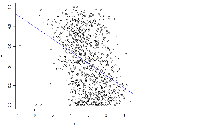
I do a linear regression using R lm function:

x = log(errors)
plot(x,y)
lm.result = lm(formula = y ~ x)
abline(lm.result, col="blue") # showing the "fit" in blue

enter image description here

but it does not fit well. Unfortunately I can't make sense of the manual.

Can someone point me in the right direction to fit this better?

By fitting I mean I want to minimize the Root Mean Squared Error (RMSE).


Edit: I have posted a related question (it's the same problem) here: Can I decrease further the RMSE based on this feature?

and the raw data here:

http://tny.cz/c320180d

except that on that link x is what is called errors on the present page here, and there are less samples (1000 vs 3000 in the present page plot). I wanted to make things simpler in the other question.

$\endgroup$
16
  • 4
    $\begingroup$ R lm works as expected, the problem is with your data, i.e. linear relationship is not apropriate in this case. $\endgroup$
    – mpiktas
    Commented Jan 28, 2014 at 7:16
  • 2
    $\begingroup$ Could you draw what line you think you should get and why you think your line has smaller MSE? I note your y's lie between 0 and 1, so it sounds like linear regression would be quite unsuitable for these data. What are the values? $\endgroup$
    – Glen_b
    Commented Jan 28, 2014 at 7:23
  • 2
    $\begingroup$ If the y values are probabilities, you don't want OLS regression at all. $\endgroup$
    – Peter Flom
    Commented Jan 28, 2014 at 10:48
  • 3
    $\begingroup$ (sorry could post this before) What looks to you like "a better fit" below is (approximately) minimizing the sums of squares of orthogonal distances, not the vertical distances' your intuition is mistaken. You can check the approximate MSE easily enough! If the y-values are probabilities, you'd be better served by some model that doesn't go outside the range 0 to 1. $\endgroup$
    – Glen_b
    Commented Jan 28, 2014 at 11:27
  • 2
    $\begingroup$ It could be that this regression suffers from the presence of a few outliers. Could be a case for robust regression. en.wikipedia.org/wiki/Robust_regression $\endgroup$ Commented Jan 29, 2014 at 20:45

5 Answers 5

19
$\begingroup$

One of the simplest solutions recognizes that changes among probabilities that are small (like 0.1) or whose complements are small (like 0.9) are usually more meaningful and deserve more weight than changes among middling probabilities (like 0.5).

For instance, a change from 0.1 to 0.2 (a) doubles the probability while (b) changing the complementary probability only by 1/9 (dropping it from 1-0.1 = 0.9 to 1-0.2 to 0.8), whereas a change from 0.5 to 0.6 (a) increases the probability only by 20% while (b) decreasing the complementary probability only by 20%. In many applications that first change is, or at least ought to be, considered to be almost twice as great as the second.

In any situation where it would be equally meaningful to use a probability (of something occurring) or its complement (that is, the probability of the something not occurring), we ought to respect this symmetry.

These two ideas--of respecting the symmetry between probabilities $p$ and their complements $1-p$ and of expressing changes relatively rather than absolutely--suggest that when comparing two probabilities $p$ and $p'$ we should be tracking both their ratios $p'/p$ and the ratios of their complements $(1-p)/(1-p')$. When tracking ratios it is simpler to use logarithms, which convert ratios into differences. Ergo, a good way to express a probability $p$ for this purpose is to use $$z = \log p - \log(1-p),$$ which is known as the log odds or logit of $p$. Fitted log odds $z$ can always be converted back into probabilities by inverting the logit; $$p = \exp(z)/(1+\exp(z)).$$ The last line of the code below shows how this is done.

This reasoning is rather general: it leads to a good default initial procedure for exploring any set of data involving probabilities. (There are better methods available, such as Poisson regression, when the probabilities are based on observing ratios of "successes" to numbers of "trials," because probabilities based on more trials have been measured more reliably. That does not seem to be the case here, where the probabilities are based on elicited information. One could approximate the Poisson regression approach by using weighted least squares in the example below to allow for data that are more or less reliable.)

Let's look at an example.

Figures

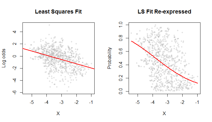
The scatterplot on the left shows a dataset (similar to the one in the question) plotted in terms of log odds. The red line is its ordinary least squares fit. It has a low $R^2$, indicating a lot of scatter and strong "regression to the mean": the regression line has a smaller slope than the major axis of this elliptical point cloud. This is a familiar setting; it is easy to interpret and analyze using R's lm function or the equivalent.

The scatterplot on the right expresses the data in terms of probabilities, as they were originally recorded. The same fit is plotted: now it looks curved due to the nonlinear way in which log odds are converted to probabilities.

In the sense of root mean squared error in terms of log odds, this curve is the best fit.

Incidentally, the approximately elliptical shape of the cloud on the left and the way it tracks the least squares line suggest that the least squares regression model is reasonable: the data can be adequately described by a linear relation--provided log odds are used--and the vertical variation around the line is roughly the same size regardless of horizontal location (homoscedasticity). (There are some unusually low values in the middle that might deserve closer scrutiny.) Evaluate this in more detail by following the code below with the command plot(fit) to see some standard diagnostics. This alone is a strong reason to use log odds to analyze these data instead of the probabilities.


#
# Read the data from a table of (X,Y) = (X, probability) pairs.
#
x <- read.table("F:/temp/data.csv", sep=",", col.names=c("X", "Y"))
#
# Define functions to convert between probabilities `p` and log odds `z`.
# (When some probabilities actually equal 0 or 1, a tiny adjustment--given by a positive
# value of `e`--needs to be applied to avoid infinite log odds.)
#
logit <- function(p, e=0) {x <- (p-1/2)*(1-e) + 1/2; log(x) - log(1-x)}
logistic <- function(z, e=0) {y <- exp(z)/(1 + exp(z)); (y-1/2)/(1-e) + 1/2}
#
# Fit the log odds using least squares.
#
b <- coef(fit <- lm(logit(x$Y) ~ x$X))
#
# Plot the results in two ways.
#
par(mfrow=c(1,2))
plot(x$X, logit(x$Y), cex=0.5, col="Gray",
     main="Least Squares Fit", xlab="X", ylab="Log odds")
abline(b, col="Red", lwd=2)

plot(x$X, x$Y, cex=0.5, col="Gray",
     main="LS Fit Re-expressed", xlab="X", ylab="Probability")
curve(logistic(b[1] + b[2]*x), col="Red", lwd=2, add=TRUE)
$\endgroup$
3
  • $\begingroup$ Thank you very much for the answer. I will need some time to try that. $\endgroup$ Commented Jan 28, 2014 at 16:21
  • $\begingroup$ I run into an error when trying your code with my data, when trying to fit the log odds: "Error in lm.fit(x, y, offset = offset, singular.ok = singular.ok, ...) : NA/NaN/Inf in foreign function call (arg 4)". $\endgroup$ Commented Jan 30, 2014 at 5:51
  • $\begingroup$ Please read the comments in the code: they explain what the problem is and what to do about it. $\endgroup$
    – whuber
    Commented Jan 30, 2014 at 16:36
8
$\begingroup$

Given the skew in the data with x, the obvious first thing to do is use a logisitic regression (wiki link). So I am with whuber on this. I will say that $x$ on its own will show strong significance but not explain away most of the deviance (the equivalent of total sum of squares in an OLS). So one might suggest that there is another covariate apart from $x$ that aids explanatory power (e.g. the people doing the classification or the method used), Your $y$ data is already [0,1] though: do you know if they represent probabilities or occurrence ratios ? If so, you should try a logistic regression using your non-transformed $y$ (before they are ratios/probabilities).

Peter Flom's observation only makes sense if your y is not a probability. Check plot(density(y));rug(y) at different buckets of $x$ and see if you see a changing Beta distribution or simply run betareg. Note that the beta distribution is also an exponential family distribution and thus it should be possible to model it with glm in R.

To give you an idea of what I meant by logistic regression:

# the 'real' relationship where y is interpreted as the probability of success
y = runif(400)
x = -2*(log(y/(1-y)) - 2) + rnorm(400,sd=2) 
glm.logit=glm(y~x,family=binomial); summary(glm.logit) 
plot(y ~ x); require(faraway); grid()
points(x,ilogit(coef(glm.logit) %*% rbind(1.0,x)),col="red")
tt=runif(400)  # an example of your untransformed regression
newy = ifelse(tt < y, 1, 0)
glm.logit=glm(newy~x,family=binomial); summary(glm.logit) 

# if there is not a good match in your tail probabilities try different link function or oversampling with correction (will be worse here, but perhaps not in your data)
glm.probit=glm(y~x,family=binomial(link=probit)); summary(glm.probit)
glm.cloglog=glm(y~x,family=binomial(link=cloglog)); summary(glm.cloglog)
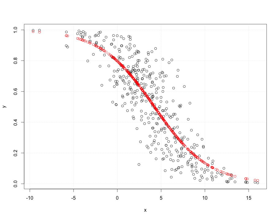
A logistic regression where the true model is $log(\frac{p}{1-p})=2-0.5x

EDIT: after reading the comments:

Given that "The y values are probabilities of being of a certain class, obtained from averaging classifications done manually by people," I strongly recommend doing a logistic regression on your base data. Here is an example:

Assume you are looking at the probability of someone agreeing to a proposal ($y=1$ agree, $y=0$ disagree) given an incentive $x$ between 0 and 10 (could be log transformed, e.g. remuneration). There are two people proposing the offer to candidates ("Jill and Jack"). The real model is that candidates have a base acceptance rate and that increases as the incentive increases. But it also depends on who is proposing the offer (in this case we say Jill has a better chance than Jack). Assume that combined they ask 1000 candidates and collect their accept (1) or reject (0) data.

require(faraway)
people = c("Jill","Jack")
proposer = sample(people,1000,replace=T)
incentive = runif(1000, min = 0, max =10)
noise = rnorm(1000,sd=2)
# base probability of agreeing is about 12% (ilogit(-2))
agrees = ilogit(-2 + 1*incentive + ifelse(proposer == "Jill", 0 , -0.75) + noise) 
tt = runif(1000)
observedAgrees = ifelse(tt < agrees,1,0)
glm.logit=glm(observedAgrees~incentive+proposer,family=binomial); summary(glm.logit) 

From the summary you can see that the model fits quite well. The deviance is $\chi^2_{n-3}$ (std of $\chi^2$ is $\sqrt{2.df}$). Which fits and it beats a model with a fixed probability (difference in deviances is several hundred with $\chi^2_{2}$). It is a bit harder to draw given that there are two covariates here but you get the idea.

xs = coef(glm.logit) %*% rbind(1,incentive,as.factor(proposer))
ys = as.vector(unlist(ilogit(xs)))
plot(ys~ incentive, type="n"); require(faraway); grid()
points(incentive[proposer == "Jill"],ys[proposer == "Jill"],col="red")
points(incentive[proposer == "Jack"],ys[proposer == "Jack"],col="blue")
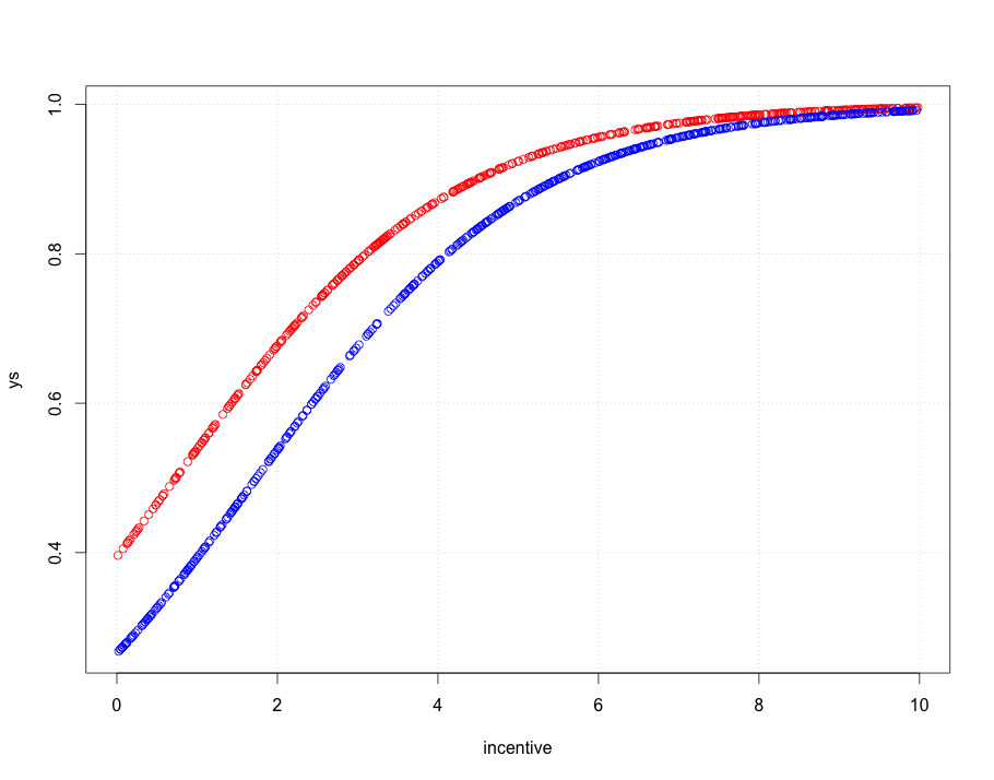
Jill in Red Jack in Blue

As you can see Jill has an easier time getting a good hit rate than Jack but that goes away as the incentive goes up.

You should basically apply this type of model to your original data. If your output is binary, keep the 1/0 if it is multinomial you need a multinomial logistic regression. If you think the extra source of variance is not the data collector, add another factor (or continuous variable) whatever you think makes sense for your data. The data comes first, second and third, only then does the model come into play.
$\endgroup$
3
  • $\begingroup$ A comment by the OP, "The y values are probabilities of being of a certain class, obtained from averaging classifications done manually by people," suggests that logistic regression would be inappropriate for these data--although it might be a great solution for the raw data (as suggested in your first paragraph), depending on what the "classifications" are and how the "averaging" occurred. When applied to the data shown in the question, glm produces a relatively flat uncurved line that looks remarkably like the line shown in the question. $\endgroup$
    – whuber
    Commented Jan 28, 2014 at 16:18
  • $\begingroup$ Thank you. And yes, y is a probability. I also posted the raw data in a related question: stats.stackexchange.com/questions/83576/…, although I called x what I called log(x) in the other question... $\endgroup$ Commented Jan 28, 2014 at 16:19
  • $\begingroup$ I wish I had known that before I acquired a sample from your image, LOL! $\endgroup$
    – whuber
    Commented Jan 28, 2014 at 16:24
6
$\begingroup$

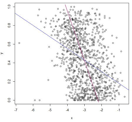
The linear regression model is not well suited for the data. One might expect to get something like the following out of the regression:

enter image description here

but by realizing what OLS does, it is obvious that this is not what you will get. A graphical interpretation of ordinary least squares is that it minimizes the squared vertical distance between the line (hyperplane) and your data. Obviously the purple line I've superimposed has some huge residuals from $x\in (-7,4.5)$ and again on the other side of 3. This is why the blue line is a better fit than the purple.

$\endgroup$
3
  • $\begingroup$ @pkofod Yes, I see. So I deleted my comment (I knew you knew it was squared; but other readers might not). $\endgroup$
    – Peter Flom
    Commented Jan 28, 2014 at 10:50
  • 2
    $\begingroup$ Censored regression is different from regression with a dependent variable that is confined to a fixed known range. These data are not censored and censored regression will do nothing different with them than ordinary regression. $\endgroup$
    – whuber
    Commented Jan 28, 2014 at 18:59
  • $\begingroup$ Yeah, my bad. Deleted that part. $\endgroup$
    – pkofod
    Commented Jan 28, 2014 at 22:22
5
$\begingroup$

Since Y is bounded by 0 and 1, ordinary least squares regression is not well-suited. You could try beta regression. In R there is the betareg package.

Try something like this

install.packages("betareg")
library(betareg)
betamod1 <- betareg(y~x, data = DATASETNAME)

more info

EDIT: If you'd like a full account of beta regression, its advantages and disadvantages, see A better lemon squeezer: Maximum likelihood regression with beta distributed dependent variables by Smithson and Verkuilen

$\endgroup$
9
  • 4
    $\begingroup$ What model is betareg actually implementing? What are its assumptions and why is it reasonable to suppose they apply to these data? $\endgroup$
    – whuber
    Commented Jan 28, 2014 at 14:59
  • 2
    $\begingroup$ @whuber It's a good question! The model is defined on pages 3 and 4 of this vignette. It's based on a beta density reparameterized in terms of mean and precision parameters (both of which can be modelled, each with its own link function), and a set of link functions the same as those used for binomial models (and one more). It's fitted by ML, and works very like fitting a GLM. $\endgroup$
    – Glen_b
    Commented Jan 30, 2014 at 6:38
  • 2
    $\begingroup$ @whuber Conditional beta models are common for compositional data and other continuous-type proportions or probabilities. I don't know whether the assumptions for such models are suitable for these data (I don't know what the data are, which would be my first concern before suggesting a model myself), but even just from the plot, I imagine that they'd fit as well as other suggested models here. There a number of models in answers here which don't seem to be any better justified than Peter's suggestion, some with (not always stated) assumptions that look to be more difficult to justify. $\endgroup$
    – Glen_b
    Commented Jan 30, 2014 at 21:39
  • 1
    $\begingroup$ Thank you, @Glen_b. I'm not challenging Peter's suggestion--only trying to understand it, because I have not used beta regression before, and I imagine many future readers would be in the same situation. (I am familiar enough with the other models mentioned in this thread to understand their assumptions and possible shortcomings!) It would therefore be nice to see this answer include at least a short account of the assumptions and the reasons for recommending this solution. $\endgroup$
    – whuber
    Commented Jan 30, 2014 at 21:56
  • 1
    $\begingroup$ Ah, yes, I've linked to that paper in an answer myself at one point. Smithson (one of the authors) has the paper up on his webpage. Supplemental material is linked here. $\endgroup$
    – Glen_b
    Commented Jan 30, 2014 at 22:23
1
$\begingroup$

You might first want to know exactly what a linear model does. It tries to model a relationship of the form

$$Y_i = a + bX_i + \epsilon_i$$

Where the $\epsilon_i$ satisfy certain conditions (heteroskedasticity, uniform variance and independence - wikipedia is a good start if that doesn't ring a bell). But even if these conditions are checked, there is absolutely no guarantee that this will be a "best fit" in the sense you're looking for : OLS is just trying to minimize error in the Y direction, which is what it's doing in your case, but which isn't what seems like the best fit.

If a linear model is really what you're looking for, you might try transforming your variables a little so that OLS can indeed be fitted, or just try another model altogether. You might want to look into PCA or CCA, or if you're really bent on using a linear model, try the total least squares solution, that might give a better "fit", as it allow errors in both directions.

$\endgroup$
2
  • $\begingroup$ I thought lm was looking for a "Total least squares" minimum for a linear function (a+b*x+epsilon). I am lost. $\endgroup$ Commented Jan 28, 2014 at 9:08
  • 1
    $\begingroup$ lm, as you used it, is minimizing the sum of squared residuals, i.e. $(y - a - b*x)^2$ for each data point, called OLS (ordinary least squares). I couldn't find a nice picture for linear OLS, but maybe this one is still illustrative to you. OLS is minimizing the square of the green lines, lm is doing this with a line. In comparison, look at a linear total least squares picture. $\endgroup$
    – Roland
    Commented Jan 28, 2014 at 10:06

Your Answer

By clicking “Post Your Answer”, you agree to our terms of service and acknowledge you have read our privacy policy.

Not the answer you're looking for? Browse other questions tagged or ask your own question.