Just because the five-number summary is identical doesn't mean that the distribution is identical. This tells you just how much information is lost when we present data graphically in a box plot!
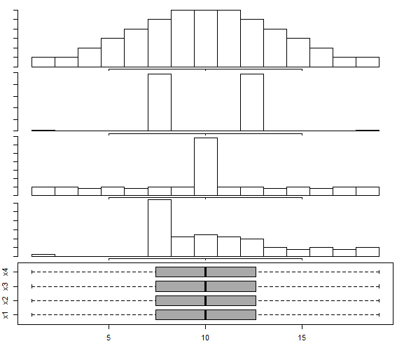
Perhaps the easiest way to see the problem is that the five number summary tells you nothing about the distribution of the values between the minimum and lower quartile, or between the lower quartile and the median, and so on. You know that the frequency between minimum and lower quartile must match the frequency between lower quartile and median (with the obvious exceptions, e.g. if we have data lying on a quartile, or worse, if two quartiles are tied) but don't know to which values of the variable those frequencies are allocated. We can have a situation like this:

These two distributions have the same five-number summary, so their box plots are identical, but I have chosen $X$ to have a uniform distribution between each quartile whereas $Y$ has a distribution with low frequencies close to the quartiles and high frequencies in the middle of two quartiles. Effectively the distribution of $Y$ has been formed by taking the distribution of $X$ and moving most of the data that is close to a quartile further away from it; my R code actually performs this in reverse, starting with the irregular distribution of $Y$ and levelling out the frequencies by reallocating data from the peaks to fill in the troughs.
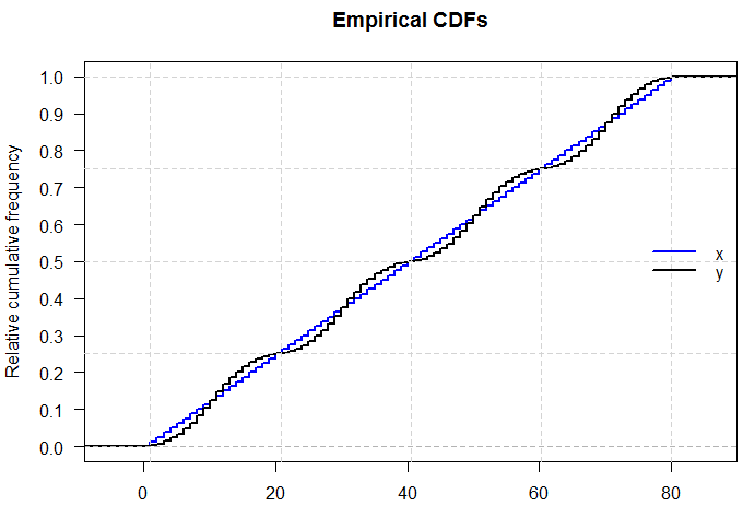
EDIT: As @Glen_b says, this becomes even more obvious when you look at the cumulative distributions. I've added gridlines to show the location of the quartiles, which are the same for the two distributions so their empirical CDFs intersect.

R code
yfreq <- 2*rep(c(1:10, 10:1), times=4)
xfreq <- rep(mean(yfreq), times=length(yfreq))

x <- rep(1:length(xfreq), times=xfreq)
y <- rep(1:length(yfreq), times=yfreq)

ecdfX <- ecdf(x)
ecdfY <- ecdf(y)
plot(ecdfX, verticals=TRUE, do.points=FALSE, col="blue", lwd=2, yaxt="n",
    main="Empirical CDFs", xlab="", ylab="Relative cumulative frequency")
plot(ecdfY, verticals=TRUE, do.points=FALSE, add=TRUE, col="black",
    yaxt="n", lwd=2)
axis(side=2, at=seq(0, 1, by=0.1), las=2)
abline(h=c(0.25,0.5,0.75,1), col="lightgrey", lty="dashed")
abline(v=summary(x), col="lightgrey", lty="dashed")
legend("right", c("x", "y"), col = c("blue", "black"),
       lty = "solid", lwd=2, bty="n")

par(mfrow=c(2,2))
hist(x, col="steelblue", breaks=((0:81)-0.5), ylim=c(0,25))
hist(y, col="grey", breaks=((0:81)-0.5), ylim=c(0,25))
boxplot(x, col="steelblue", main="Boxplot of x")
boxplot(y, col="grey", main="Boxplot of y")

summary(x)
#   Min. 1st Qu.  Median    Mean 3rd Qu.    Max.
#   1.00   20.75   40.50   40.50   60.25   80.00

summary(y)
#   Min. 1st Qu.  Median    Mean 3rd Qu.    Max.
#   1.00   20.75   40.50   40.50   60.25   80.00


