When combining p-values, why not just averaging?

Question

I recently learned about Fisher's method to combine p-values. This is based on the fact that p-value under the null follows a uniform distribution, and that $$-2\sum_{i=1}^n{\log X_i} \sim \chi^2(2n), \text{ given } X \sim \text{Unif}(0,1)$$ which I think is genius. But my question is why going this convoluted way? and why not (what is wrong with) just using mean of p-values and use central limit theorem? or median? I am trying to understand the genius of RA Fisher behind this grand scheme.

Answer 1

You can perfectly use the mean $p$-value.

Fisher’s method set sets a threshold $s_\alpha$ on $-2 \sum_{i=1}^n \log p_i$, such that if the null hypothesis $H_0$ : all $p$-values are $\sim U(0,1)$ holds, then $-2 \sum_i \log p_i$ exceeds $s_\alpha$ with probability $\alpha$. $H_0$ is rejected when this happens.

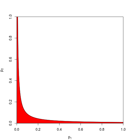
Usually one takes $\alpha = 0.05$ and $s_\alpha$ is given by a quantile of $\chi^2(2n)$. Equivalently, one can work on the product $\prod_i p_i$ which is lower than $e^{-s_\alpha/2}$ with probability $\alpha$. Here is, for $n=2$, a graph showing the rejection zone (in red) (here we use $s_\alpha = 9.49$. The rejection zone has area = 0.05.

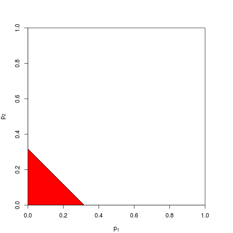
Now you can chose to work on ${1\over n} \sum_{i=1}^n p_i$ instead, or equivalently on $\sum_i p_i$. You just need to find a threshold $t_\alpha$ such that $\sum p_i$ is below $t_\alpha$ with probability $\alpha$; exact computation $t_\alpha$ is tedious – for $n$ big enough you can rely on central limit theorem; for $n = 2$, $t_\alpha = (2\alpha)^{1\over 2}$. The following graph shows the rejection zone (area = 0.05 again).

As you can imagine, many other shapes for the rejection zone are possibles, and have been proposed. It is not a priori clear which is better – i.e. which has greater power.

Let‘s assume that $p_1$, $p_2$ come from a bilateral $z$-test with non-centrality parameter 1 :

> p1 <- pchisq( rnorm(1e4, 1, 1)**2, df=1, lower.tail=FALSE )
> p2 <- pchisq( rnorm(1e4, 1, 1)**2, df=1, lower.tail=FALSE )

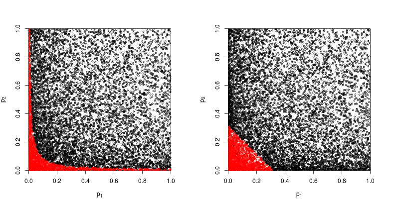
Let's have a look on the scatterplot with in red the points for which the null hypothesis is rejected.

The power of Fisher’s product method is approximately

> sum(p1*p2<exp(-9.49/2))/1e4
[1] 0.2245

The power of the method based on the sum of $p$-values is approximately

> sum(p1+p2<sqrt(0.1))/1e4
[1] 0.1963

So Fisher’s method wins – at least in this case.

Answer 2

What is wrong with summing up all individual $p$-values?

As @whuber and @Glen_b argue in the comments, Fisher's method is essentially multiplying all individual $p$-values, and multiplying probabilities is a more natural thing to do than adding them.

Still one can add them up. In fact, precisely this was suggested by Edgington (1972) An additive method for combining probability values from independent experiments (under pay-wall), and is sometimes referred to as Edgington's method. The 1972 paper concludes claiming that

The additive method is shown to be more powerful than the multiplicative method, having a greater probability than the multiplicative method of yielding significant results when there actually are treatment effects.

but given that the method remains relatively unknown, I suspect that this was at least an oversimplification. E.g. a recent overview Cousins (2008) Annotated Bibliography of Some Papers on Combining Significances or p-values does not mention Edgington's method at all and it seems that this term has never been mentioned on CrossValidated either.

It is easy to come up with various ways of combining $p$-values (I have once come up with one myself and asked why it is never used: Stouffer's Z-score method: what if we sum $z^2$ instead of $z$?), and what is a better method is largely an empirical question. Please see @whuber's answer there for an empirical comparison of statistical power of two different methods in a specific situation; there is a clear winner.

So the answer to the general question about why using any "convoluted" method at all, is that one can gain power.

Zaykin et al (2002) Truncated Product Method for Combining p-values runs some simulations and includes Edgington's method in the comparison, but I am not sure about the conclusions.

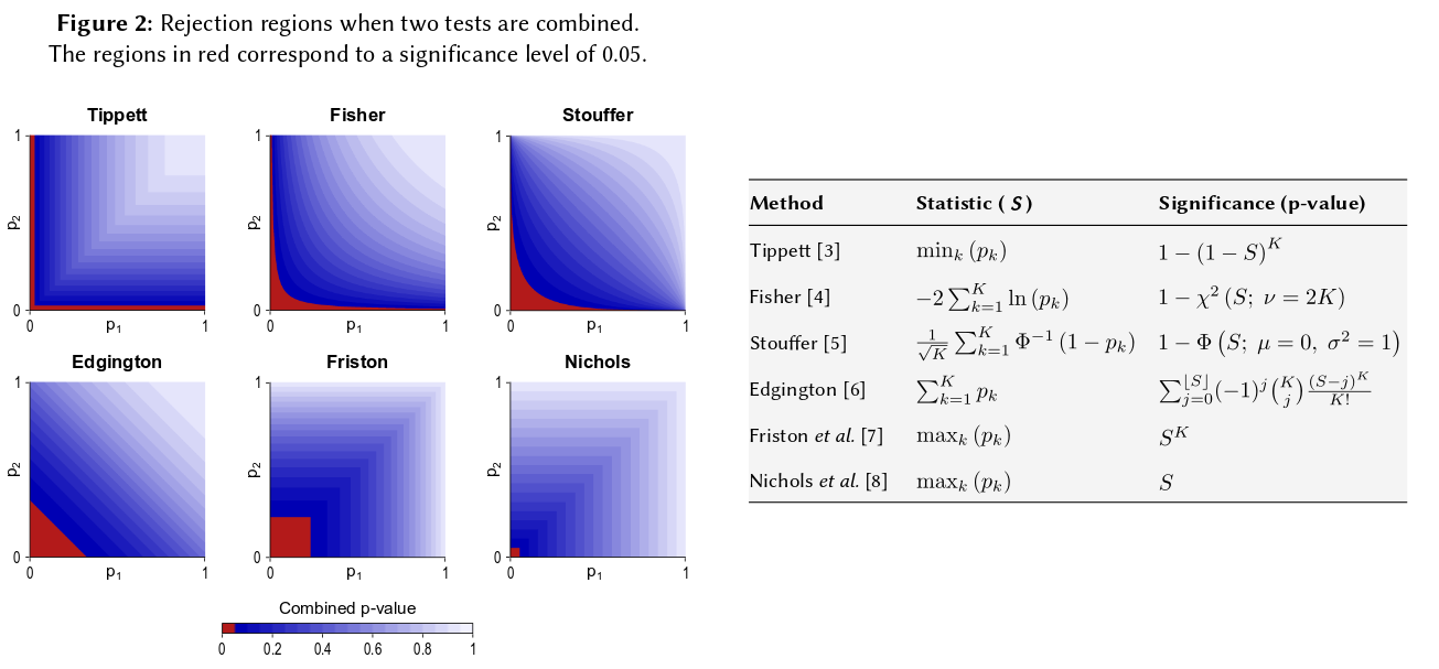
One way to visualize all such methods is to draw rejection regions for $n=2$, as @Elvis did in his nice answer (+1). Here is another figure that explicitly includes Edgington's method from what appears to be a poster Winkler et al (2013) Non-Parametric Combination for Analyses of Multi-Modal Imaging:

Having said all that, I think there still remains a question of why Edgington's method would (often?) be suboptimal, as follows from it being obscure.

Perhaps one reason for obscurity is that it does not conform to our intuition very well: for $n=2$, if $p_1 = 0.4$ (or higher) then no matter what the value of $p_2$ is, the combined null will not be rejected at $\alpha=0.05$, that is even if e.g. $p_2 = 0.00000001$.

More generally, summing $p$-values hardly distinguishes very small numbers like e.g. $p=0.001$ from $p=0.00000001$, but the difference in these probabilities is actually huge.

---

Update. Here is what Hedges and Olkin write about Edgintgon's method (after reviewing other methods for combining $p$-values) in their Statistical Methods for Meta-Analysis (1985), emphasis mine:

A quite different combined test procedure was proposed by Edgington (1972a,b). Edgington proposed combining $p$-values by taking the sum $$S = p_1 + \cdots + p_k,$$ and gave a tedious but straightforward method for obtaining significance levels for $S$. A large sample approximation to the significance levels of $S$ is given in Edgington (1972b). Although it is a monotone combination pro­cedure and therefore is admissible, Edgington's method is generally thought to be a poor procedure since one large $p$-value can overwhelm many small values that compose the statistic. However, there have been almost no numerical investigations of this procedure.

Answer 3

So if you did three studies of similar sizes and got a p-value of 0.05 on all three occasions, your intuition is that the "true value" should be 0.05? My intuition is different. Multiple similar results would seem to make the significance higher (and therefore the p-values which are probabilities should be lower). P-values are not really probabilities. They are statements about the sample distribution of observed values under a particular hypothesis. I believe that it may have given support to the notion that one can misuse them as such. I regret making that assertion.

At any rate, under the null hypothesis of no difference, the chances of getting multiple extreme p-values would seem to be much more unlikely. Every time I see the statement that the p-value is uniformly distributed from 0-1 under the null hypothesis I feel compelled to test it with simulation, and so far the statement seems to hold. I'm apparently do not think consciously on a logarithmic scale, although at least part of my cerebral neural net must.

If you want to quantify this intuition, the formula you offered (with slight revisions) appears in the Wikipedia page: http://en.wikipedia.org/wiki/Fisher%27s_method , and the associated graphic lets you quantify visually and semi-quantitatively the impact of getting two small p-values on the overall significance. For example reading from the color coded graphic, 2 simultaneous p-values of 0.05 would give a synthetic p-value around .02. You could also investigate the impact on the t-statistics of doubling your sample size. The sample size enters into the sample t-statistic as 1/sqrt(n-1) so you could look at the impact of that factor as a result of going from 50 to 100. (in R:)

 plot(1:100, 1/sqrt(1:100) ,ylim=c(0,1) )
 abline(h=1/sqrt(c(50,100)))

Those two approaches yield different quantitative results, since the ratio the 1/sqrt(n) values for 50 and 100 are not the same as the ratio of 0.05 to 0.02. Both approaches support my intuition, but to different degrees. Maybe someone else can resolve this discrepancy. Yet a third approach would be to consider the probability of getting two random draws of "True" when the binomial probability of each draw was .05. (an extremely unfair dice) That joint event should have a probability of .05*.05=.002, which result could be considered on the "other side" of the Fisher estimate. I just ran a simulation of 50,000 simultaneous t.tests. If you plot the results it looks very much like the maps of the cosmic background radiation field... ie. mostly random.

 t1 <- replicate(50000, t.test(rnorm(50))$p.value )
     t2 <- replicate(50000, t.test(rnorm(50))$p.value )
 table(t1 < 0.05, t2 < 0.05)
 plot(t1, t2, cex=0.1)
#        FALSE  TRUE
#  FALSE 45099  2411
#  TRUE   2380   110
 110/(50000-110)
#[1] 0.002204851