Why L1 norm for sparse models

Question

I am reading books about linear regression. There are some sentences about the L1 and L2 norm. I know the formulas, but I don't understand why the L1 norm enforces sparsity in models. Can someone give a simple explanation?

Answer 1

Consider the vector $\vec{x}=(1,\varepsilon)\in\mathbb{R}^2$ where $\varepsilon>0$ is small. The $l_1$ and $l_2$ norms of $\vec{x}$, respectively, are given by

$$\Vert \vec{x}\Vert_1 = 1+\varepsilon,\ \ \Vert\vec{x}\Vert_2^2 = 1+\varepsilon^2$$

Now say that, as part of some regularization procedure, we are going to reduce the magnitude of one of the elements of $\vec{x}$ by $\delta\leq\varepsilon$. If we change $x_1$ to $1-\delta$, the resulting norms are

$$\Vert\vec{x}-(\delta,0)\Vert_1 = 1-\delta+\varepsilon,\ \ \Vert\vec{x}-(\delta,0)\Vert_2^2 = 1-2\delta+\delta^2+\varepsilon^2$$

On the other hand, reducing $x_2$ by $\delta$ gives norms

$$\Vert\vec{x}-(0,\delta)\Vert_1 = 1-\delta+\varepsilon,\ \ \Vert\vec{x}-(0,\delta)\Vert_2^2 = 1-2\varepsilon\delta+\delta^2+\varepsilon^2$$

The thing to notice here is that, for an $l_2$ penalty, regularizing the larger term $x_1$ results in a much greater reduction in norm than doing so to the smaller term $x_2\approx 0$. For the $l_1$ penalty, however, the reduction is the same. Thus, when penalizing a model using the $l_2$ norm, it is highly unlikely that anything will ever be set to zero, since the reduction in $l_2$ norm going from $\varepsilon$ to $0$ is almost nonexistent when $\varepsilon$ is small. On the other hand, the reduction in $l_1$ norm is always equal to $\delta$, regardless of the quantity being penalized.

Another way to think of it: it's not so much that $l_1$ penalties encourage sparsity, but that $l_2$ penalties in some sense discourage sparsity by yielding diminishing returns as elements are moved closer to zero.

Answer 2

With a sparse model, we think of a model where many of the weights are 0. Let us therefore reason about how L1-regularization is more likely to create 0-weights.

Consider a model consisting of the weights $(w_1, w_2, \dots, w_m). $

With L1 regularization, you penalize the model by a loss function $L_1(w) = \sum_i |w_i|.$

With L2-regularization, you penalize the model by a loss function $L_2(w) = \frac{1}{2} \sum_i w_i^2.$

If using gradient descent, you will iteratively make the weights change in the opposite direction of the gradient with a step size $\eta$ multiplied with the gradient. This means that a more steep gradient will make us take a larger step, while a more flat gradient will make us take a smaller step. Let us look at the gradients (subgradient in case of L1):

$\frac{dL_1(w)}{dw} = \operatorname{sign}(w)$, where $\operatorname{sign}(w) := \left(\frac{w_1}{|w_1|}, \frac{w_2}{|w_2|}, \dots, \frac{w_m}{|w_m|}\right),$

$\frac{dL_2(w)}{dw} = w. $

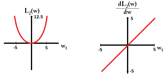
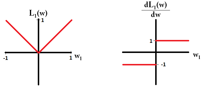
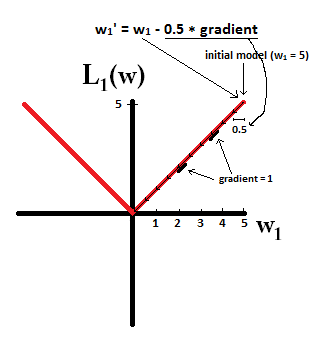
If we plot the loss function and it's derivative for a model consisting of just a single parameter, it looks like this for L1:

And like this for L2:

Notice that for $L_1$, the gradient is either 1 or -1, except for when $w_1 = 0$. That means that L1-regularization will move any weight towards 0 with the same step size, regardless the weight's value. In contrast, you can see that the $L_2$ gradient is linearly decreasing towards 0 as the weight goes towards 0. Therefore, L2-regularization will also move any weight towards 0, but it will take smaller and smaller steps as a weight approaches 0.

Try to imagine that you start with a model with $w_1 = 5$ and using $\eta = \frac{1}{2}$. In the following picture, you can see how gradient descent using L1-regularization makes 10 of the updates $w_1 := w_1 - \eta \cdot \frac{dL_1(w)}{dw} = w_1 - \frac{1}{2} \cdot 1$, until reaching a model with $w_1 = 0$:

In constrast, with L2-regularization where $\eta = \frac{1}{2}$, the gradient is $w_1$, causing every step to be only halfway towards 0. That is, we make the update $w_1 := w_1 - \eta \cdot \frac{dL_2(w)}{dw} = w_1 - \frac{1}{2} \cdot w_1$ Therefore, the model never reaches a weight of 0, regardless of how many steps we take:

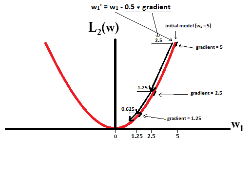
Note that L2-regularization can make a weight reach zero if the step size $\eta$ is so high that it reaches zero in a single step. Even if L2-regularization on its own over or undershoots 0, it can still reach a weight of 0 when used together with an objective function that tries to minimize the error of the model with respect to the weights. In that case, finding the best weights of the model is a trade-off between regularizing (having small weights) and minimizing loss (fitting the training data), and the result of that trade-off can be that the best value for some weights are 0.

Answer 3

The Figure 3.11 from Elements of Statistical Learning by Hastie, Tibshirani, and Friedman is very illustrative: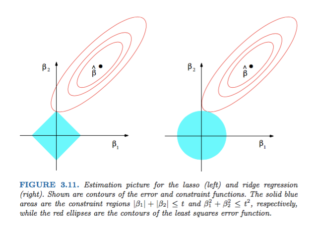

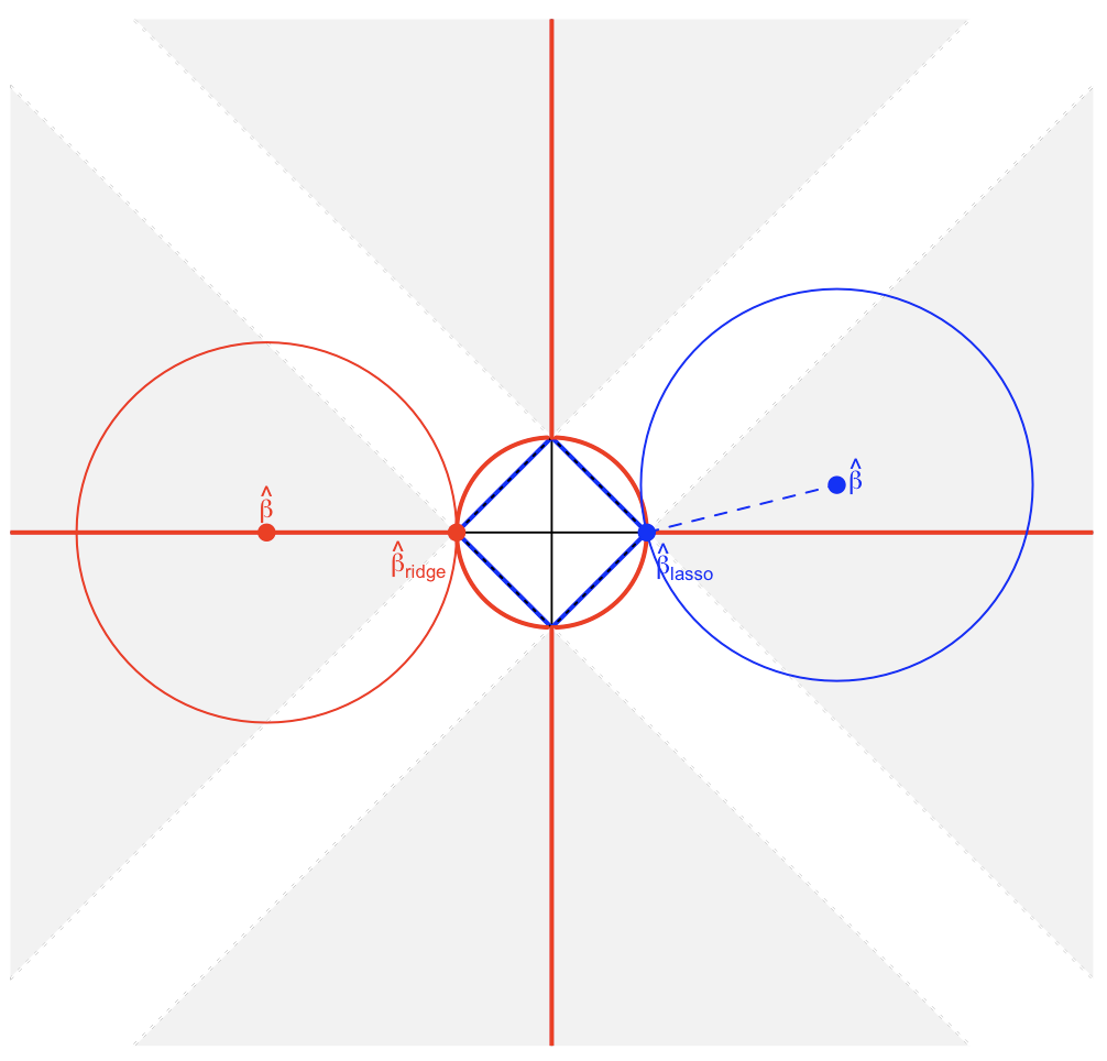
Explanations: The $\hat{\beta}$ is the unconstrained least squares estimate. The red ellipses are (as explained in the caption of this Figure) the contours of the least squares error function, in terms of parameters $\beta_1$ and $\beta_2$. Without constraints, the error function is minimized at the MLE $\hat{\beta}$, and its value increases as the red ellipses out expand. The diamond and disk regions are feasible regions for lasso ($L_1$) regression and ridge ($L_2$) regression respectively. Heuristically, for each method, we are looking for the intersection of the red ellipses and the blue region as the objective is to minimize the error function while maintaining the feasibility.

That being said, it is clear to see that the $L_1$ constraint, which corresponds to the diamond feasible region, is more likely to produce an intersection that has one component of the solution is zero (i.e., the sparse model) due to the geometric properties of ellipses, disks, and diamonds. It is simply because diamonds have corners (of which one component is zero) that are easier to intersect with the ellipses that extending diagonally. To make this intuition a little more formal, consider the scenario that the design matrix $X$ is column-wise orthogonal (i.e., $X^\top X = I_{(p)}$), under which case the LASSO problem has a closed-form solution (see this answer for the proof): $$\hat{\beta}_j^{\text{LASSO}} = \operatorname{sgn}(\hat{\beta}_j)(|\hat{\beta}_j| - \gamma)^+, \; j = 1, 2, \ldots, p.$$

Geometrically (when $p = 2$, and $\hat{\beta}$ is outside feasible regions), any $\hat{\beta}$ that falls in the gray-shaded region (call it $A_L$) in the plot below would result in a sparse LASSO solution. By contrast, only those $\hat{\beta}$ that falls on the red-colored lines on axes (call it $A_R$) in the plot below could result in a sparse ridge solution. The blue and red circles in the plot are two sample contours of error functions (note that because $X$ is column-wise orthogonal, the contours are circular instead of elliptical -- this is also why we can delineate the exact $\hat{\beta}$-region resulting in sparse LASSO solutions) for a sparse LASSO solution $\hat{\beta}_{\text{lasso}}$ and a sparse ridge solution $\hat{\beta}_{\text{ridge}}$.

In fact, for this special scenario, we can claim that the probability of getting a sparse LASSO solution is positive while the probability of getting a sparse ridge solution is zero: since the 2D-Lebesgue measure of $A_L$ is positive while that of $A_R$ is zero, and (under the assumption that errors are i.i.d. $N(0, \sigma^2)$) $\hat{\beta} \sim N_2(\beta, \sigma^2 I_{(2)})$, it follows that \begin{align*} & P(\hat{\beta}_{\text{lasso}} \text{ is sparse}) = P(\hat{\beta} \in A_L) = \frac{1}{\sigma^2}\iint_{A_L}\phi\left(\frac{x - \beta_1}{\sigma}\right)\phi\left(\frac{y - \beta_2}{\sigma}\right)dxdy > 0, \\ & P(\hat{\beta}_{\text{ridge}} \text{ is sparse}) = P(\hat{\beta} \in A_R) = \frac{1}{\sigma^2}\iint_{A_R}\phi\left(\frac{x - \beta_1}{\sigma}\right)\phi\left(\frac{y - \beta_2}{\sigma}\right)dxdy = 0. \end{align*} To some extent, this provides a mathematical proof to why it is easier to get a sparse LASSO solution than to get a sparse ridge solution.

Answer 4

Have a look on figure 3.11 (page 71) of The elements of statistical learning. It shows the position of a unconstrained $\hat \beta$ that minimizes the squared error function, the ellipses showing the levels of the square error function, and where are the $\hat \beta$ subject to constraints $\ell_1 (\hat \beta) < t$ and $\ell_2 (\hat \beta) < t$.

This will allow you to understand very geometrically that subject to the $\ell_1$ constraint, you get some null components. This is basically because the $\ell_1$ ball $\{ x : \ell_1(x) \le 1\}$ has "edges" on the axes.

More generally, this book is a good reference on this subject: both rigorous and well illustrated, great explanations.

Answer 5

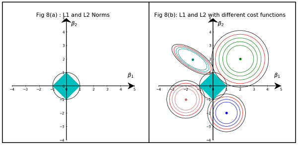
The image shows the shapes of area occupied by L1 and L2 Norm. The second image consists of various Gradient Descent contours for various regression problems. In all the contour plots, observe the red circle which intersects the Ridge or L2 Norm. the intersection is not on the axes. The black circle in all the contours represents the one which interesects the L1 Norm or Lasso. It intersects relatively close to axes. This results in making coefficients to 0 and hence feature selection. Hence L1 norm make the model sparse.

More Detailed explanation at the following link: Click Post on Towards Data Science

Answer 6

A simple non mathematical answer wold be:

For L2: Penalty term is squared,so squaring a small value will make it smaller. We don't have to make it zero to achieve our aim to get minimum square error, we will get it before that.

For L1: Penalty term is absolute,we might need to go to zero as there are no catalyst to make small smaller.

This my point of view.

Answer 7

I suggest you read some more about the theory of convex optimization. An answer to why the $ \ell_1 $ regularization achieves sparsity can be found if you examine implementations of models employing it, for example LASSO. One such method to solve the convex optimization problem with $ \ell_1 $ norm is by using the proximal gradient method, as $ \ell_1 $ norm is not differentiable. I found Ryan Tibshirani's slides for his convex optimization course to be quite helpful on this topic, even though my mathematical background is limited.

You can find the derivation of the soft-thresholding operator $ S_\lambda $ used in the slides in the first answer to the mathematics StackExchange question on deriving the soft-thresholding operator. It is not too hard to follow, even without great knowledge of subgradients, and its result clearly shows why you get sparsity--for some $ \lambda > 0 $, for the $ i $th component $ w_t^i $ of the weight vector at time $ t $, the proximal gradient step is $ w_{t + 1}^i = w_t^i - \lambda $ if $ |w_t^i| > \lambda $, $ w_{t + 1}^i = 0 $ when $ |w_t^i| \le \lambda $. In ISTA (iterative soft-thresholding algorithm) described in Tibshirani's slides for LASSO, you would see that the weight vector update is

$$ \mathbf{w}_{t + 1} = S_\lambda(\mathbf{w}_t + \eta\mathbf{X}^\top(\mathbf{y} - \mathbf{X}\mathbf{w})) $$

That is, after the least-squares gradient update with step $ \eta > 0 $, you perform soft-thresholding. This achieves sparsity, as the vector components with magnitude less than $ \lambda $ are set to 0.

You can replace $ -\mathbf{X}^\top(\mathbf{y} - \mathbf{Xw}) $ with a general objective function gradient as well.

Answer 8

l2 regularizer does not change the value of weight vector from one iteration to another iteration because of the slope of l2 norm is reducing all the time where as l1 regularizer constantly reduce the value of weight vector towards optimal W* which is 0 because of the slopeod L1 norm is constant