Paired t-test results

Question

I'm running a paired t-test to compare before and after counts. Here's what my data looks like:

before <- c(102,122,64,0)
after <- c(38,39,23,16)

Here's my results of the t.test:

t.test(before, after, data = fence2016.data, paired = TRUE)
    Paired t-test

data:  before and after
t = 2.0038, df = 3, p-value = 0.1388
alternative hypothesis: true difference in means is not equal to 0
95 percent confidence interval:
 -25.29295 111.29295
sample estimates:
mean of the differences 
                     43 

I'm wondering why my p-value isn't that significant? The count data obviously changes significantly between before and after. Is there another parameter I should be using? I want to prove that there is a significant difference between before and after (hopefully a negative difference too).

Answer 1

The sample size is very low and the variance is very large. Meaning that although the average difference is pretty large (and positive, actually), such a thing can still happen by accident if there is no real difference. So in fact your result is correct and your intuition is wrong. The differences are not significant. ("Insignificant" means that the data are compatible with the null hypothesis, and actually they are. Obviously that doesn't mean that the null hypothesis is true.)

"Is there another parameter I should be using? I want to prove that there is a significant difference between before and after (hopefully a negative difference too)."

No, you have done the right thing, so all you can do is to accept a result that apparently you don't like. Note by the way that trying out another test because you didn't like the result of the first one will be invalid, whatever test you use, because the theory behind tests doesn't allow for the test you run to be chosen conditionally on the data.

Answer 2

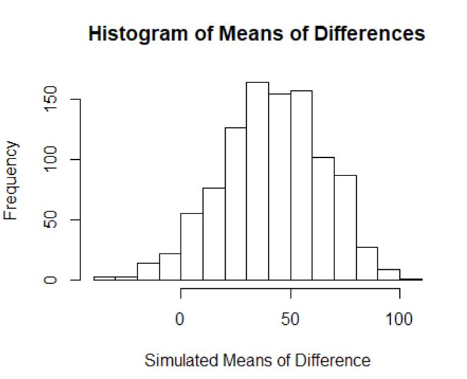
The other answers are more direct and just better. But here is another perspective. This answer is probably wrong (whether it is correct or not depends on the nature of you data), but one that will help you see what's going on. One idea is that we can treat your data like its own population, and sample repeatedly from it (with replacement). This is known as bootstrapping. If we do that many times and take the mean of the differences, what does the distribution of those simulations look like? In fact, about 4.5% of the time, it will be on the negative side (depending on how you do the difference). Why is this technically wrong? It is probably not correct to say that your pairs are interchangeable. For example, the 102 observation is probably coming from a different distribution as compared to your 0 observation from the "before" data set. This is why the interval below is so different from R's.

    #Load in data
    before <- c(102,122,64,0)
    after <- c(38,39,23,16)

    #Specify how many bootstraps you want to do.
    simulations<-1000
    simulation_results<-data.frame(mean_of_diffs=rep(NA,simulations))

    #Bootstrap
    for(i in 1:simulations){
      simulation_results$mean_of_diffs[i]<-mean(sample(x = before,size = length(before),replace = T)-sample(x = after,size = length(after),replace = T))
    }

    #Compare with a plot
    hist(simulation_results$mean_of_diffs,main = "Histogram of Means of Differences",xlab = "Simulated Means of Difference")

    #Get an empirical confidence interval
    quantile(simulation_results$mean_of_diffs,probs = c(.025,.975))

Answer 3

Without being too rigourous, the p-value you see is dependent on

1. how many samples you have, and
2. the variability of these samples.

The paired differences you have are (-64, -83, -41, +16), which varies by quite a bit. Together with the low number of data points, the test is telling you that it is still quite possible to see these sampled paired difference by chance when the before and after count is the same (which is what you assumed in the statistical test to start with).

A comparable (again, non-rigourous) situation is that you are flipping a fair coin, the difference between the times you have heads and tails should not be different in the long run, but it is quite plausible that you end up with 3H/1T or 3T/1H in your first four coin flips.

The OP should consider having more paired difference samples, or find some way to reduce the variability of the sampled pair differences if the goal is for future iterations to achieve statistical significance. Without full context of the underlying data generation process the latter will be difficult though. Standard warnings about p-hacking applies.