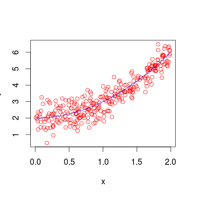
I'm using R to fit a neural network to data generated by the formula $y = x^2 + \frac{\epsilon}{2}$ where $x \sim \mathcal{U}(0, 2)$ and $\epsilon \sim N(0, 1)$ (very simple, right?). The following plot shows the plot of function $x^2$ and the generated data:

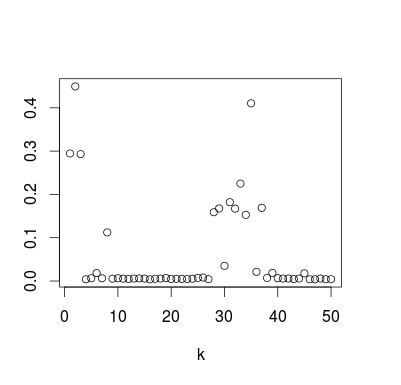
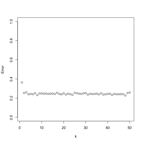
Now, I take the average error for $10$ runs for a Neural Network model of size $k$ for all $k \in \{1, \ldots, 50\}$ getting the following plot:

What I find rather strange is that from ~$10$ to ~$30$ and from ~$40$ to ~$50$ it is $\approx 0$ and stable but from ~$30$ to ~$40$ it is volatile and $>> 0$. I've also tried several other functions getting the same effect. Is that normal? Can you provide an explanation for it?
The plot above was generated by the following R code:
require(nnet)

f<-function(x) 2 + x^2

error <- rep(0, 50)

for (k in 1:50) {
  for (z in 1:10) {
    x<-sort(runif(300,0,2))
    fx <- f(x)
    y<-fx + 0.5*rnorm(300)
    d<-data.frame(x,y)
    names(d)<-c("X","Y")

    n<-nnet(Y~X,size=k,linout=T,data=d,maxit=40)
    pn<-predict(n,d)

    error[k] = error[k] + mean((fx - pn)^2)
  }
  error[k] = error[k] / 10
  plot(error, xlab = "k", ylab = "Error")
}

