Estimating adjusted risk ratios in binary data using Poisson regression

Question

I am interested in estimating an adjusted risk ratio, analogous to how one estimates an adjusted odds ratio using logistic regression. Some literature (e.g., this) indicates that using Poisson regression with Huber-White standard errors is a model-based way to do this

I have not found literature on how adjusting for continuous covariates affects this. The following simple simulation demonstrates that this issue is not so straightforward:

arr <- function(BLR,RR,p,n,nr,ce)
{
   B = rep(0,nr)
   for(i in 1:nr){
   b <- runif(n)<p 
   x <- rnorm(n)
   pr <- exp( log(BLR) + log(RR)*b + ce*x)
   y <- runif(n)<pr
   model <- glm(y ~ b + x, family=poisson)
   B[i] <- coef(model)[2]
   }
   return( mean( exp(B), na.rm=TRUE )  )
}

set.seed(1234)
arr(.3, 2, .5, 200, 100, 0)
[1] 1.992103
arr(.3, 2, .5, 200, 100, .1)
[1] 1.980366
arr(.3, 2, .5, 200, 100, 1)
[1] 1.566326 

In this case, the true risk ratio is 2, which is recovered reliably when the covariate effect is small. But, when the covariate effect is large, this gets distorted. I assume this arises because the covariate effect can push up against the upper bound (1) and this contaminates the estimation.

I have looked but have not found any literature on adjusting for continuous covariates in adjusted risk ratio estimation. I am aware of the following posts on this site:

• Poisson regression to estimate relative risk for binary outcomes
• Poisson regression for binary data

but they do not answer my question. Are there any papers on this? Are there any known cautions that should be exercised?

Answer 1

I don't know if you still need an answer to this question, but I have a similar problem in which I'd like to use Poisson regression. In running your code, I found that if I set up the model as

model <- glm(y ~ b + x, family=binomial(logit)

rather than as your Poisson regression model, the same result occurs: the estimated OR is ~1.5 as ce approaches 1. So, I'm not sure that your example provides information on a possible problem with the use of Poisson regression for binary outcomes.

Answer 2

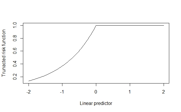
I find that using direct maximum likelihood with the proper probability function greatly improves estimation of the relative risk. You can directly specify the truncated risk function as the predicted rate for the process.

Usually we use the Hessian to create CIs for the estimate. I have not explored the possibility of using that as the "B" matrix (meat) in the Huber White error and using the fitted risks to get the "A" matrix (bread)... but I suspect it could work! More feasibly you can use a bootstrap to obtain model errors which are robust to a misspecified mean-variance relationship.

## the negative log likelihood for truncated risk function
negLogLik <- function(best, X, y) { 
  pest <- pmin(1, exp(X %*% best))
  -sum(dpois(x = y, lambda = pest, log=TRUE))
}

set.seed(100)

sim <- replicate(100, {
  n <- 200
  X <- cbind(1, 'b'=rbinom(n, 1, 0.5), 'x'=rnorm(n))
  btrue <- c(log(0.3), log(2), 1)
  ptrue <- pmin(1, exp(X %*% matrix(btrue)))
  y <- rbinom(n, 1, ptrue) ## or just take y=ptrue for immediate results
  nlm(f = logLik, p = c(log(mean(y)),0,0), X=X, y=y)$estimate
})

rowMeans(exp(sim))

Gives:

> rowMeans(exp(sim))
[1] 0.3002813 2.0680780 3.0888280

The middle coefficient gives you what you want.