3
$\begingroup$

I have two dependent variables y1 and y2 with highly skewed distributions. In order to do ANOVA, I was trying to transform the data to normality.

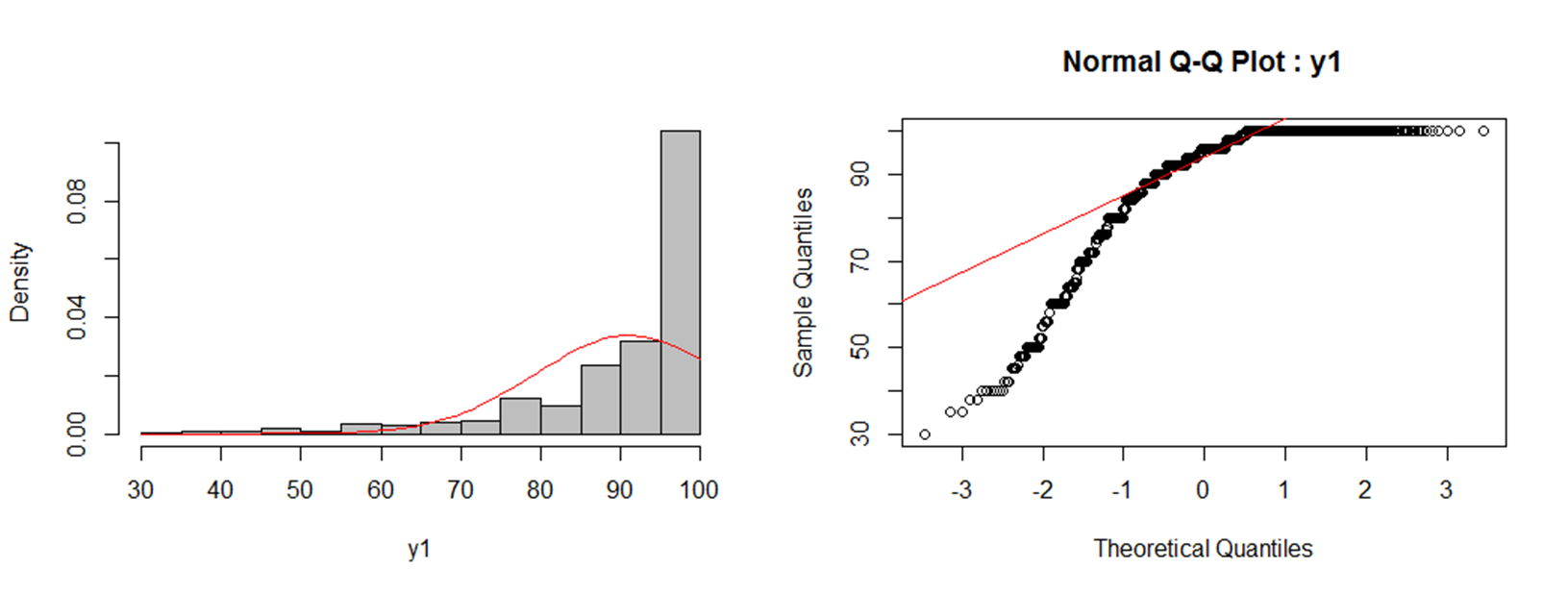
enter image description here

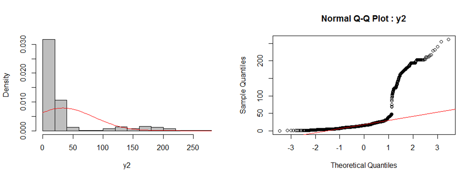
enter image description here

y1 is a proportion expressed as percentage.

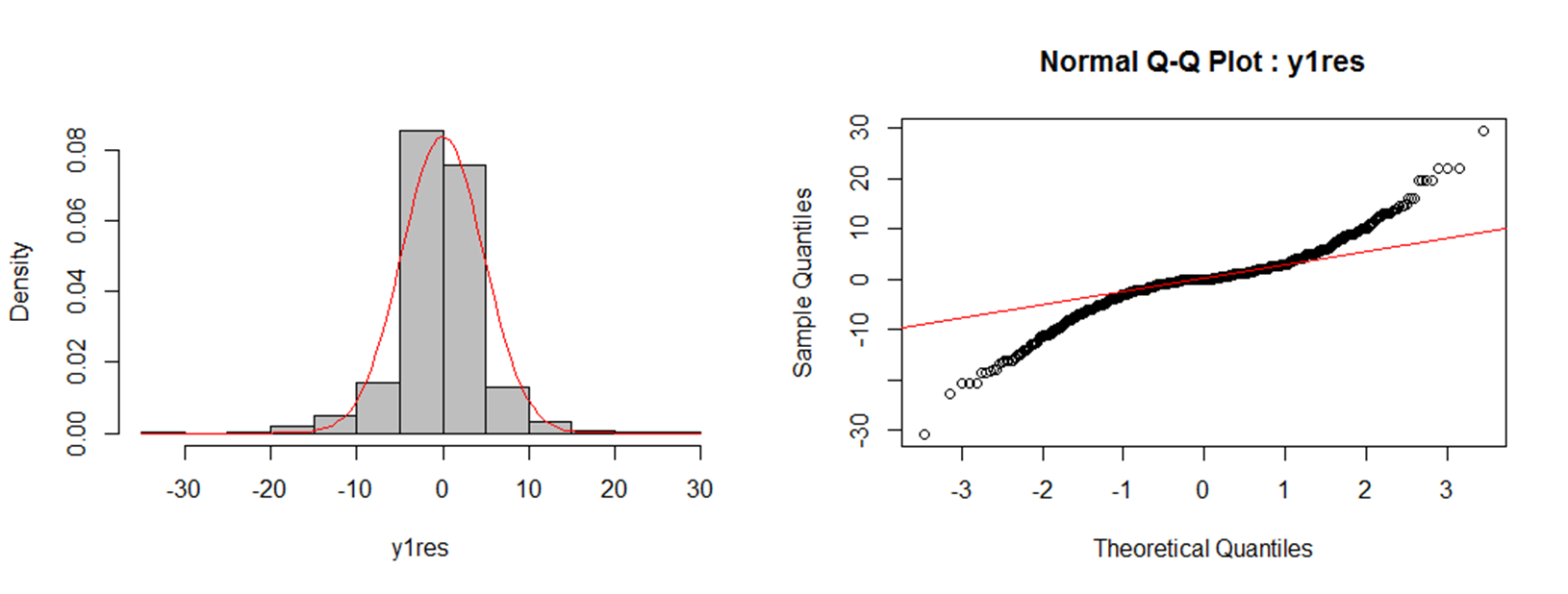
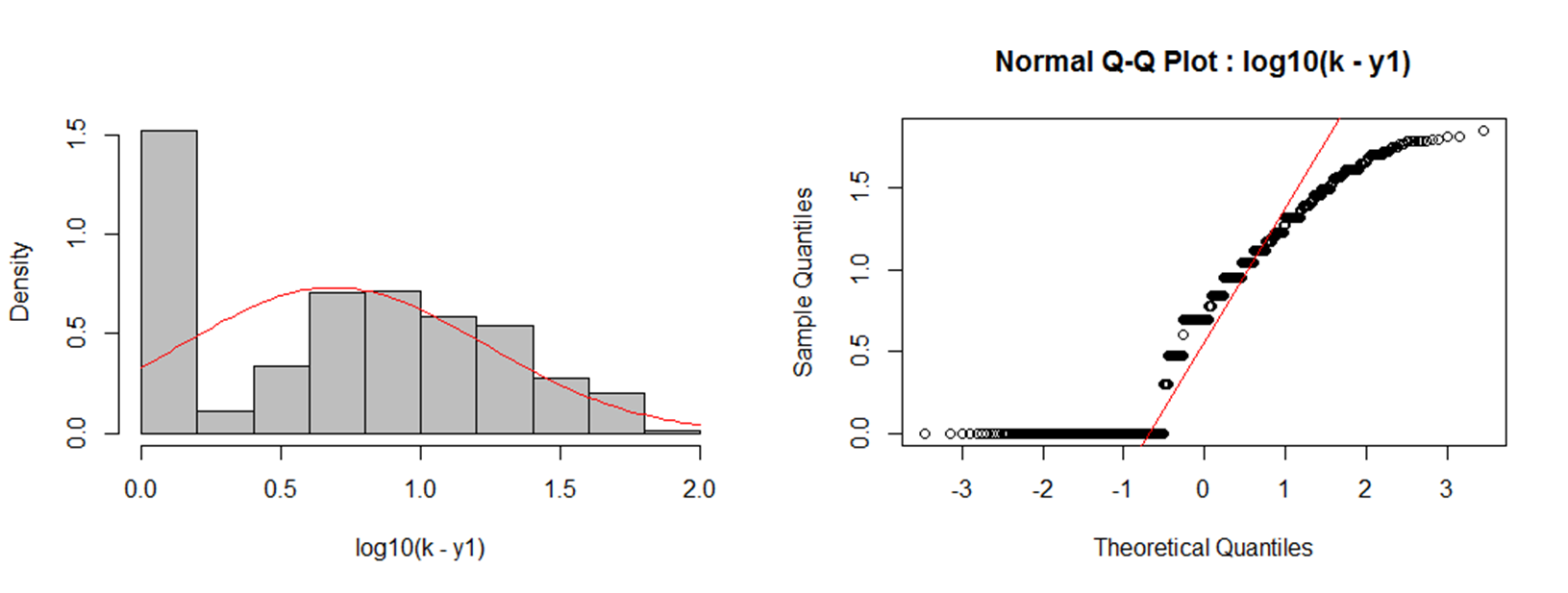
For y1 I tried log of reflected data. log10(k - y1), where k = max(y1) + 1. enter image description here

y1 being a proportion, I also tried a logit transformation. log(y1/(100 - y1)). However, there were many Inf values.

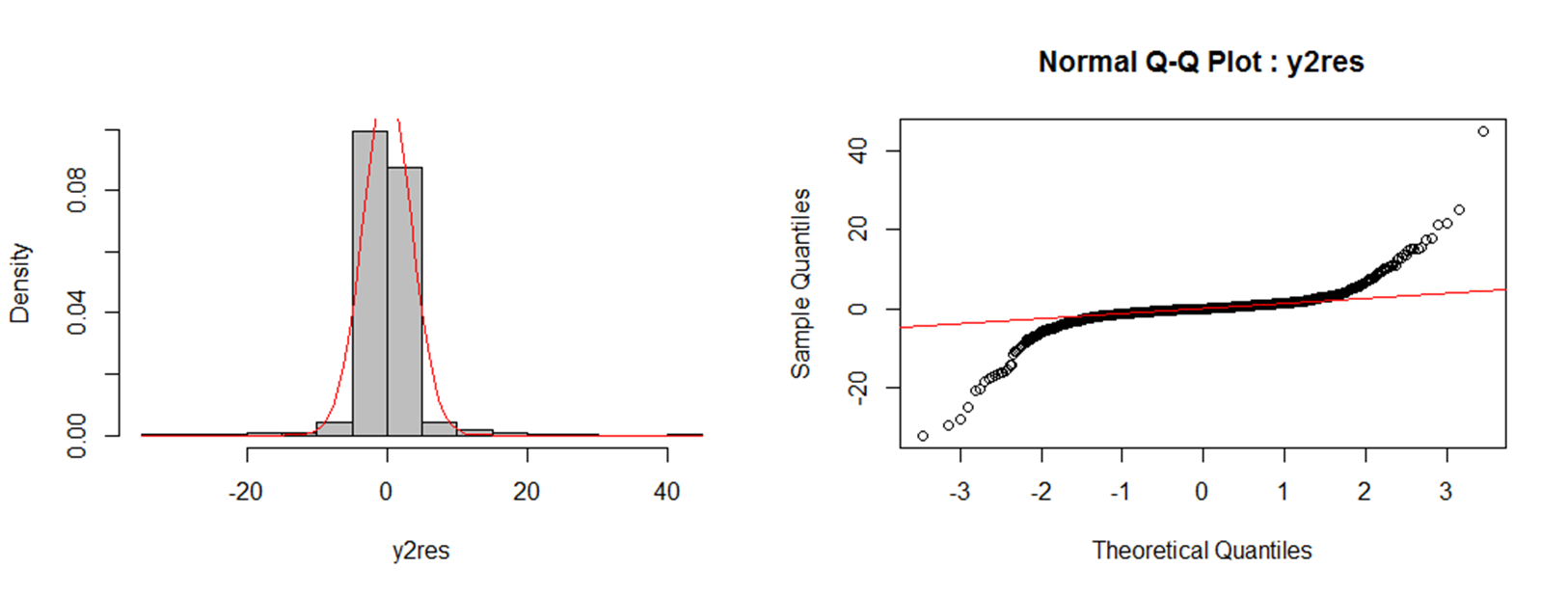
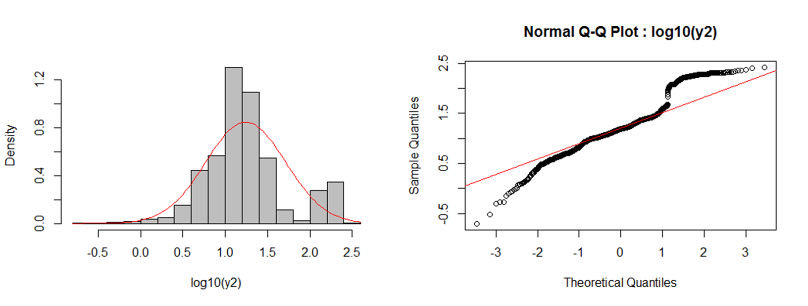
For y2 I tried log10 of the data. enter image description here

The residuals of the ANOVA model in both the cases are heavy tailed distributions.

enter image description here

enter image description here

Should I transform the data for ANOVA? If so, what is the most appropriate strategy?

$\endgroup$
1
  • 3
    $\begingroup$ The distributions very well could be skewed due to how the dependent variables depend on the independent variables. There is no assumption in ANOVA that the dependent variable is Normal! (This is a very, very frequent FAQ.) Thus you shouldn't even be performing such an analysis in the first place. $\endgroup$
    – whuber
    Commented Jul 5, 2016 at 13:33

4 Answers 4

10
$\begingroup$

As @Glen_b comments, neither distribution is (very) suitable for transformation.

General comments

Here's a Golden Rule in Feynmanesque style, except that there's a Leaden Rule Corollary that is sufficient to sink many misguided hopes in this territory.

Golden Rule With a transformation, the same values map to the same values. Several values of 1? Necessarily their logarithm is the same at 0. Several values of 49? Necessarily their square root is the same at 7.

Leaden Rule Corollary A spike in the original will always be a spike when transformed. A spike here is a large bunch of identical values in the original data. It follows that no transformation will remove a spike. No exceptions! You can move a spike closer to the main mass of the data (or further away; that can happen too). You can't remove it.

A spike often occurs at a limiting value, say a minimum or maximum, at which values pile up.

But there can be other kinds of examples. See Why do a density plot and a rug plot seem to disagree? for an extraordinary example with a famous dataset that is easy to miss if you don't look carefully enough at the data.

So spikes in the middle of a distribution are possible too. Sometimes there is a spike of exact 0s among negative, zero and positive values as a side-effect of data resolution or some algorithm. These spikes look worse than they behave, on the whole.

But what about almost identical values? That depends. A really strong transformation can work wonders, but always check, preferably graphically. For example, a logit transformation of beta distributions always yields a unimodal result, even with so-called U-shaped distributions.

Specific comments on the data examples

In this case, a percent measure with values at either 0 or 100 or both such as y1 is hard to transform. Reflection is useless, as it just reflects the problem. Logit transformation is useless if either bound is attained. Some people try folded power (such as folded root or cube root) transformations. On those see e.g.

Regression: Scatterplot with low R squared and high p-values

What is the most appropriate way to transform proportions when they are an independent variable?

and their references. (The second has comments on the often treacherous $\log($value $+$ smidgen$)$.)

A percent measure, even a measure with values at 0 and/or 100, can however be response variable in a generalized linear model with logit link. That assumes only that means are defined on the logit scale. The fact that logits of 0 and 1 (100%) are undefined need not bite.

More widely, note that with ANOVA the key assumption focused on is that conditional distributions are normal. Marginal normality is irrelevant as such. And ANOVA will often work quite well if outliers are absent. Clearly, you need to consider other assumptions too, all of them more important than normality.

I would probably work with logarithms of y2, or better with a generalized linear model with logarithmic link. You will need to look carefully to see what's behind the bimodality.

Yet more general comments

The question here, like many others on transformation, focuses on marginal normality as a goal of transformation. That goal can be unattainable (bad news, supposedly) but not nearly so important as people imagine (good news, immediately), even for methods such as regression and ANOVA widely thought to require normality. It is worth underlining that transformation can have many goals, such as the diffuse but crucial goal of helping you to see the structure in the data, or the lack of structure, even though that lack will be unwanted and disappointing.

This answer gives no worked examples (the OP did not post data) but the threads linked above all contain examples.
$\endgroup$
2
  • $\begingroup$ From you suggestions, it seems that a GLM is more appropriate for the data, with link functions logit for y1 and log for y2. But in such a case what should be the distibution to be specified in dist= in SAS GENMOD or family argument in R glm(). $\endgroup$
    – Crops
    Commented Jul 8, 2016 at 10:24
  • 2
    $\begingroup$ I've never used SAS and only occasionally use R. Software-specific questions are off-topic here, but in software I know of binomial family and robust standard errors should work reasonably. Some people call that quasi-binomial. $\endgroup$
    – Nick Cox
    Commented Jul 8, 2016 at 12:14
7
$\begingroup$
  1. ANOVA makes no assumption about the marginal distribution of the response, so transforming before looking at the residuals will leaving you trying to solve a problem you don't have (and solving the wrong one when you do have one).

  2. When you have a lot of observations all at one value (as you do with $y_1$), no transformation will separate those values. So the conditional distribution will not be normal and cannot be made normal.

Attempting a transformation to normality is not usually a suitable approach for proportions and is useless for proportions that have a spike of values at exactly 0 or 1.

What kind of proportions are these? Count proportions? Mixing proportions (like the fraction of land that is desert or the proportion of molecule A in some mixture)?

Rather than trying to force these into ANOVA, you will do better to start with trying to figure out suitable models for these kinds of variables, from which an ANOVA-like analysis can be done.

$\endgroup$
4
  • $\begingroup$ Written while mine was written; our main message unsurprisingly is similar. I disagree marginally about proportions that can be exactly 0 or 1. $\endgroup$
    – Nick Cox
    Commented Jul 5, 2016 at 9:14
  • $\begingroup$ @Nick It's possible I mistake your intent ... if there's a spike of values at 0 or 1, just as we have here... what transformation would produce normality? ... Oh, perhaps it's my phrasing that's the issue -- you actually need to have a substantive spike rather than just the possibility of one. $\endgroup$
    – Glen_b
    Commented Jul 5, 2016 at 9:53
  • 2
    $\begingroup$ We both know the answer: none of them. To me transformation is mostly a way of making structure in the data easier to see and to analyse (or lack of structure, as the case may be). The specific goal of marginal normal distributions is overstated and, precisely that, a specific goal of transformation. We've both said as much many times here, you probably many times yet than me. The linked threads in my answer show cases where folded powers make things clearer, as much as one can hope in many problems. I will think about adding further comments to my answer. $\endgroup$
    – Nick Cox
    Commented Jul 5, 2016 at 9:59
  • 1
    $\begingroup$ (Apparent disagreement resolved by editing, but I've left my comments in place, as the exchange goes a little further than the question.) $\endgroup$
    – Nick Cox
    Commented Jul 5, 2016 at 11:22
4
$\begingroup$

Your transformations are unlikely to be successful for the following reasons:

1) For y1, the majority of values are identical and equal to 100. Especially because y1 is bounded between 0 and 100, you are probably better off using a Beta distribution instead of a normal distribution.

2) For y2, your data looks like a mixture of two normal distributions (on the log scale). The big gap between 50 and 100 (on the untransformed data) is a bit of a tip off, and it's quite clear on the log plot. While Box-Cox transformations (as recommended by @Ian_Fin) are very useful in many cases, you may be better off using a mixture model here to characterize both distributions.

Also, as a general tip: your histograms are too coarse to show what is going on in the data very well. Try using more breaks to improve this, e.g. hist(y1, breaks = 50) , or use a kernel density plot with a smoothing value estimated from the data.

$\endgroup$
4
  • 1
    $\begingroup$ Kernel density plots need extra special care over what is done at either extreme. For the first data example, that could obscure as much as illuminate. Kernel estimation often obscures genuine spikes, in other words. The quantile-quantile plots tell the full story. $\endgroup$
    – Nick Cox
    Commented Jul 5, 2016 at 9:18
  • 1
    $\begingroup$ On behalf of Boxes and Coxes everywhere, I underline that Box and Cox are proper names. $\endgroup$
    – Nick Cox
    Commented Jul 5, 2016 at 9:18
  • $\begingroup$ Fair points, @NickCox $\endgroup$
    – mkt
    Commented Jul 5, 2016 at 9:22
  • 1
    $\begingroup$ Pedantic note: in y1 I don't think it's quite a majority at 100%. This is clearer on the quantile plots. Your advice is unaffected. $\endgroup$
    – Nick Cox
    Commented Jul 5, 2016 at 9:22
0
$\begingroup$

The boxcoxfit() function in the R package geoR uses a maximum likelihood approach to estimate an appropriate value of $\lambda$ for a Box-Cox transformation. No guarantee that the transformation will make your data normal, but in my experience it tends to perform quite well.

Alternatively, you may need to look into non-parametric approaches. Without knowing more about your independent variables I can't suggest which they may more appropriate.

https://cran.r-project.org/web/packages/geoR/ https://en.wikipedia.org/wiki/Power_transform#Box.E2.80.93Cox_transformation

$\endgroup$
2
  • 4
    $\begingroup$ Neither of these distributions will be rendered close to normal by any power transformation. The first has a spike, so no transformation can work. The second has at least two modes. $\endgroup$
    – Glen_b
    Commented Jul 5, 2016 at 8:50
  • $\begingroup$ Also, the boxcox transform is better at stabilizing variance than it is at normalizing! $\endgroup$ Commented Feb 23, 2017 at 21:03

Your Answer

By clicking “Post Your Answer”, you agree to our terms of service and acknowledge you have read our privacy policy.

Not the answer you're looking for? Browse other questions tagged or ask your own question.